---
title: "Predicting Arabica and Robusta Coffee Futures Prices: A Machine Learning Approach with Macroeconomic, Climatic, and Speculative Determinants"
subtitle: "Master's Thesis in Management — Business Analytics Orientation"
author: "Mohamed Hussein"
date: today
institution: "HEC Lausanne, University of Lausanne (UNIL)"
supervisor: "M. Vialfont"
format:
html:
toc: true
toc-depth: 3
number-sections: true
theme: cosmo
code-fold: true
code-summary: "Show code"
code-tools: true
css: styles.css
lang: en
---
# Data
## Setup
This chunk initialises the working environment for the entire pipeline. All file paths and global constants are defined here and referenced in every subsequent chunk, so that no hard-coded paths appear elsewhere in the document. Constructing all paths relative to `BASE_PATH` ensures full reproducibility across machines: relocating the data folder requires editing a single line.
```{r setup, message=FALSE, warning=FALSE}
packages_requis <- c(
  "readxl", "dplyr", "tidyr", "lubridate", "zoo", "readr",
  "ggplot2", "corrplot", "tseries", "urca", "forecast",
  "scales", "gridExtra", "knitr", "kableExtra", "moments",
  "ggrepel", "randomForest", "xgboost", "e1071", "nnet",
  "Metrics", "tibble"
)
for (pkg in packages_requis) {
  if (!requireNamespace(pkg, quietly = TRUE)) {
    install.packages(pkg, dependencies = TRUE)
  }
}
invisible(lapply(packages_requis, library, character.only = TRUE))


# ----------------------------------------------------------
# ROOT AND SUBDIRECTORY PATHS
# BASE_PATH points to the data folder at the project root.
# All subdirectories are derived from it using file.path(),
# so moving the data folder only requires editing one line.
# ----------------------------------------------------------

BASE_PATH        <- "Datasets mémoire de master"
PATH_CLIMATIQUES <- file.path(BASE_PATH, "Climatiques")
PATH_PRECIP      <- file.path(BASE_PATH, "Climatiques", "Précipitations")
PATH_TEMP        <- file.path(BASE_PATH, "Climatiques", "Températures")
PATH_REFINITIV   <- file.path(BASE_PATH, "Extraction Refinitiv")
PATH_MACRO       <- file.path(BASE_PATH, "Macroéconomique et financier")
PATH_COT         <- file.path(BASE_PATH, "Spéculation ICE Arabica Hebdomadaire")
PATH_OUTPUT      <- "output"

# Create output folders if they do not already exist
if (!dir.exists(PATH_OUTPUT)) dir.create(PATH_OUTPUT)
dir.create(file.path(PATH_OUTPUT, "tables"), showWarnings = FALSE)


# ----------------------------------------------------------
# INDIVIDUAL FILE PATHS — PRICE AND MACROECONOMIC DATA
# Daily futures prices are sourced from Refinitiv via CEDIF.
# Macroeconomic series are sourced from FRED, Investing.com,
# the USDA FAS PSD Online database, and the OECD.
# ----------------------------------------------------------

# Futures prices (daily, aggregated to monthly in later chunks)
FICHIER_ARABICA  <- file.path(PATH_REFINITIV, "Arabica_Coffee_Daily_Price_Refinitiv.xlsx")
FICHIER_ROBUSTA  <- file.path(PATH_REFINITIV, "Robusta_Coffee_Daily_Price_Refinitiv.xlsx")
FICHIER_CACAO_NY <- file.path(PATH_REFINITIV, "ICE_NY_Cocoa_Daily_Price_Refinitiv.xlsx")
FICHIER_SUCRE_11 <- file.path(PATH_REFINITIV, "Sugar_No.11_Daily_Price_Refinitiv.xlsx")

# Macroeconomic and fundamental variables
FICHIER_USDA <- file.path(PATH_MACRO, "Coffee_Green_Production_Consumption_Export_Yearly.xlsx")
FICHIER_CPI  <- file.path(PATH_MACRO, "Inflation_CPI_Monthly_1990.csv")
FICHIER_WTI  <- file.path(PATH_MACRO, "Prix_du_Pétrole_WTI_Monthly_1990.csv")
FICHIER_FED  <- file.path(PATH_MACRO, "Taux_Directeur_FED_Monthly_1990.csv")
FICHIER_DXY  <- file.path(PATH_MACRO, "US_DXY_Index_Monthly_Historical_Data_1990.csv")
FICHIER_PIB  <- file.path(PATH_MACRO, "Quarterly_GDP_OECD_from_2000_to_2025.xlsx")

# ENSO climate index
FICHIER_ONI  <- file.path(PATH_CLIMATIQUES, "Index_ONI_Monthly_LONG_Format_1950.xlsx")


# ----------------------------------------------------------
# CLIMATE DATA FILE LISTS — 14 PRODUCER COUNTRIES
# ERA5 reanalysis data (World Bank CCKP, ADM1 resolution)
# is stored as one file per country per climate variable.
# The list names match the internal identifiers used when
# computing production-weighted climate indices downstream.
# Only countries with an average production share >= 1%
# over 2000-2024 are retained (see chunk `selection_pays`).
# ----------------------------------------------------------

FICHIERS_PRECIP <- list(
  bresil      = file.path(PATH_PRECIP, "précipitations_brésil_1950_2023_monthly.xlsx"),
  vietnam     = file.path(PATH_PRECIP, "précipitations_vietnam_1950_2023_monthly.xlsx"),
  colombie    = file.path(PATH_PRECIP, "précipitations_colombie_1950_2023_monthly.xlsx"),
  indonesie   = file.path(PATH_PRECIP, "précipitations_indonésie_1950_2023_monthly.xlsx"),
  ethiopie    = file.path(PATH_PRECIP, "précipitations_éthiopie_1950_2023_monthly.xlsx"),
  inde        = file.path(PATH_PRECIP, "précipitations_inde_1950_2023_monthly.xlsx"),
  honduras    = file.path(PATH_PRECIP, "précipitations_honduras_1950_2023_monthly.xlsx"),
  mexique     = file.path(PATH_PRECIP, "précipitations_mexique_1950_2023_monthly.xlsx"),
  uganda      = file.path(PATH_PRECIP, "précipitations_ouganda_1950_2023_monthly.xlsx"),
  guatemala   = file.path(PATH_PRECIP, "précipitations_guatemala_1950_2023_monthly.xlsx"),
  perou       = file.path(PATH_PRECIP, "précipitations_pérou_1950_2023_monthly.xlsx"),
  cote_ivoire = file.path(PATH_PRECIP, "précipitations_côte_d_ivoire_1950_2023_monthly.xlsx"),
  nicaragua   = file.path(PATH_PRECIP, "précipitations_nicaragua_1950_2023_monthly.xlsx"),
  costa_rica  = file.path(PATH_PRECIP, "précipitations_costa_rica_1950_2023_monthly.xlsx")
)

FICHIERS_TEMP <- list(
  bresil      = file.path(PATH_TEMP, "températures_brésil_1950_2023_monthly.xlsx"),
  vietnam     = file.path(PATH_TEMP, "températures_vietnam_1950_2023_monthly.xlsx"),
  colombie    = file.path(PATH_TEMP, "températures_colombie_1950_2023_monthly.xlsx"),
  indonesie   = file.path(PATH_TEMP, "températures_indonésie_1950_2023_monthly.xlsx"),
  ethiopie    = file.path(PATH_TEMP, "températures_éthiopie_1950_2023_monthly.xlsx"),
  inde        = file.path(PATH_TEMP, "températures_inde_1950_2023_monthly.xlsx"),
  honduras    = file.path(PATH_TEMP, "températures_honduras_1950_2023_monthly.xlsx"),
  mexique     = file.path(PATH_TEMP, "températures_mexique_1950_2023_monthly.xlsx"),
  uganda      = file.path(PATH_TEMP, "températures_ouganda_1950_2023_monthly.xlsx"),
  guatemala   = file.path(PATH_TEMP, "températures_guatemala_1950_2023_monthly.xlsx"),
  perou       = file.path(PATH_TEMP, "températures_pérou_1950_2023_monthly.xlsx"),
  cote_ivoire = file.path(PATH_TEMP, "températures_côte_d_ivoire_1950_2023_monthly.xlsx"),
  nicaragua   = file.path(PATH_TEMP, "températures_nicaragua_1950_2023_monthly.xlsx"),
  costa_rica  = file.path(PATH_TEMP, "températures_costa_rica_1950_2023_monthly.xlsx")
)


# ----------------------------------------------------------
# COT FILE LIST — CFTC DISAGGREGATED FUTURES-ONLY REPORTS
# The CFTC provides one consolidated file covering June 2006
# to 2015, followed by individual annual files from 2016
# onward. All files are read and stacked in chunk `cot`.
# ----------------------------------------------------------

FICHIERS_COT <- c(
  file.path(PATH_COT, "juin_2006-2015.xls"),
  file.path(PATH_COT, "2016.xls"), file.path(PATH_COT, "2017.xls"),
  file.path(PATH_COT, "2018.xls"), file.path(PATH_COT, "2019.xls"),
  file.path(PATH_COT, "2020.xls"), file.path(PATH_COT, "2021.xls"),
  file.path(PATH_COT, "2022.xls"), file.path(PATH_COT, "2023.xls"),
  file.path(PATH_COT, "2024.xls")
)


# ----------------------------------------------------------
# GLOBAL TIME CONSTANTS
# These bounds are applied as filters in every subsequent
# chunk, ensuring strict temporal consistency across the
# entire dataset assembly and modelling pipeline.
# ----------------------------------------------------------

DATE_DEBUT     <- "2000-01"   # Start of the main analysis period
DATE_FIN       <- "2023-12"   # End of the main analysis period
DATE_DEBUT_COT <- "2006-06"   # First available COT observation (June 2006)
```
## Overview of the Dataset
This study draws on eight distinct data sources covering the period from January 2000 to December 2023, yielding 288 monthly observations for the main analysis and 96 quarterly observations for specifications that incorporate GDP growth. The analysis period begins in 2000 for three converging reasons. First, the suspension of the International Coffee Organization's export quota system in 1989 and its definitive abandonment in the early 1990s led to a decade of institutional transition, culminating in the 2001 ICO reform that established the fully liberalised price regime that prevails today. Data prior to 2000 therefore reflect a structurally different market environment and would introduce regime-change breaks that complicate time series modelling. Second, the ERA5 reanalysis dataset used for climate variables reaches its highest spatial and temporal reliability from the late 1990s onward, as the assimilation of satellite observations improves significantly over this period. Third, several key variables — including the CFTC Disaggregated COT report and Robusta futures prices from Refinitiv — are either unavailable or unreliable before this period. The analysis ends in December 2023, the last month for which all data sources are simultaneously available at the time of data collection.
This chunk produces the variable summary table presented in the text. Each row corresponds to one variable retained in the final dataset, grouped by category. The table is built manually as a data frame so that the ordering and grouping of rows can be controlled precisely, then rendered using `kableExtra` with row-merging on the Category column for readability.
```{r table_variables}
# Build the variable inventory as a structured data frame.
# Rows are ordered by category first, then by variable role
# within each category (dependent before regressors, etc.).
table_vars <- data.frame(
  Category = c(
    "Dependent", "Dependent",
    "Spillovers", "Spillovers",
    "Macroeconomic", "Macroeconomic", "Macroeconomic", "Macroeconomic",
    "Macroeconomic",
    "Fundamentals", "Fundamentals", "Fundamentals", "Fundamentals",
    "Speculation",
    "Climate", "Climate", "Climate"
  ),
  Variable = c(
    "Arabica futures price (ICE/NYBOT)",
    "Robusta futures price (LIFFE)",
    "Sugar No.11 futures price (ICE)",
    "Cocoa futures price (ICE NY)",
    "WTI crude oil price",
    "US Dollar Index (DXY)",
    "Federal Funds Rate",
    "US Consumer Price Index (CPI)",
    "OECD real GDP growth rate",
    "World coffee production",
    "World coffee consumption",
    "World coffee exports",
    "World ending stocks",
    "Managed Money net position (COT)",
    "Weighted precipitation index (14 countries)",
    "Weighted temperature index (14 countries)",
    "Oceanic Niño Index (ONI)"
  ),
  Source = c(
    "Refinitiv / CEDIF (UNIL)",
    "Refinitiv / CEDIF (UNIL)",
    "Refinitiv / CEDIF (UNIL)",
    "Refinitiv / CEDIF (UNIL)",
    "FRED (Federal Reserve)",
    "Investing.com",
    "FRED (Federal Reserve)",
    "FRED (Federal Reserve)",
    "OECD Data Explorer",
    "USDA FAS PSD Online",
    "USDA FAS PSD Online",
    "USDA FAS PSD Online",
    "USDA FAS PSD Online",
    "CFTC Disaggregated Futures-Only",
    "World Bank CCKP (ERA5 0.25°)",
    "World Bank CCKP (ERA5 0.25°)",
    "NOAA"
  ),
  Frequency = c(
    "Monthly", "Monthly (from 2008)",
    "Monthly", "Monthly",
    "Monthly", "Monthly", "Monthly", "Monthly",
    "Quarterly",
    "Annual (expanded to monthly)",
    "Annual (expanded to monthly)",
    "Annual (expanded to monthly)",
    "Annual (expanded to monthly)",
    "Monthly (from June 2006)",
    "Monthly", "Monthly", "Monthly"
  ),
  stringsAsFactors = FALSE
)

# Render the table with merged category cells and striped rows.
# collapse_rows() merges consecutive identical values in the
# Category column, avoiding visual repetition in the output.
kable(table_vars,
      caption   = "Summary of variables, sources and frequencies",
      col.names = c("Category", "Variable", "Source", "Frequency"),
      booktabs  = TRUE) %>%
  kable_styling(bootstrap_options = c("striped", "hover"),
                font_size = 11, full_width = TRUE) %>%
  collapse_rows(columns = 1, valign = "middle")
```
Two data availability constraints deserve explicit acknowledgement. First, Robusta futures prices from Refinitiv are available only from 2008 onward; the 96 months spanning 2000–2007 are therefore missing for this variable, and Robusta models are estimated on the 2008–2023 sub-period. Second, the CFTC Disaggregated COT report — which distinguishes Managed Money from commercial traders — was introduced in June 2006. The net speculative position variable accordingly contains missing values for the 2000–2006 period, which is documented and handled in the modelling phase.
## Dependent Variables: Coffee Futures Prices
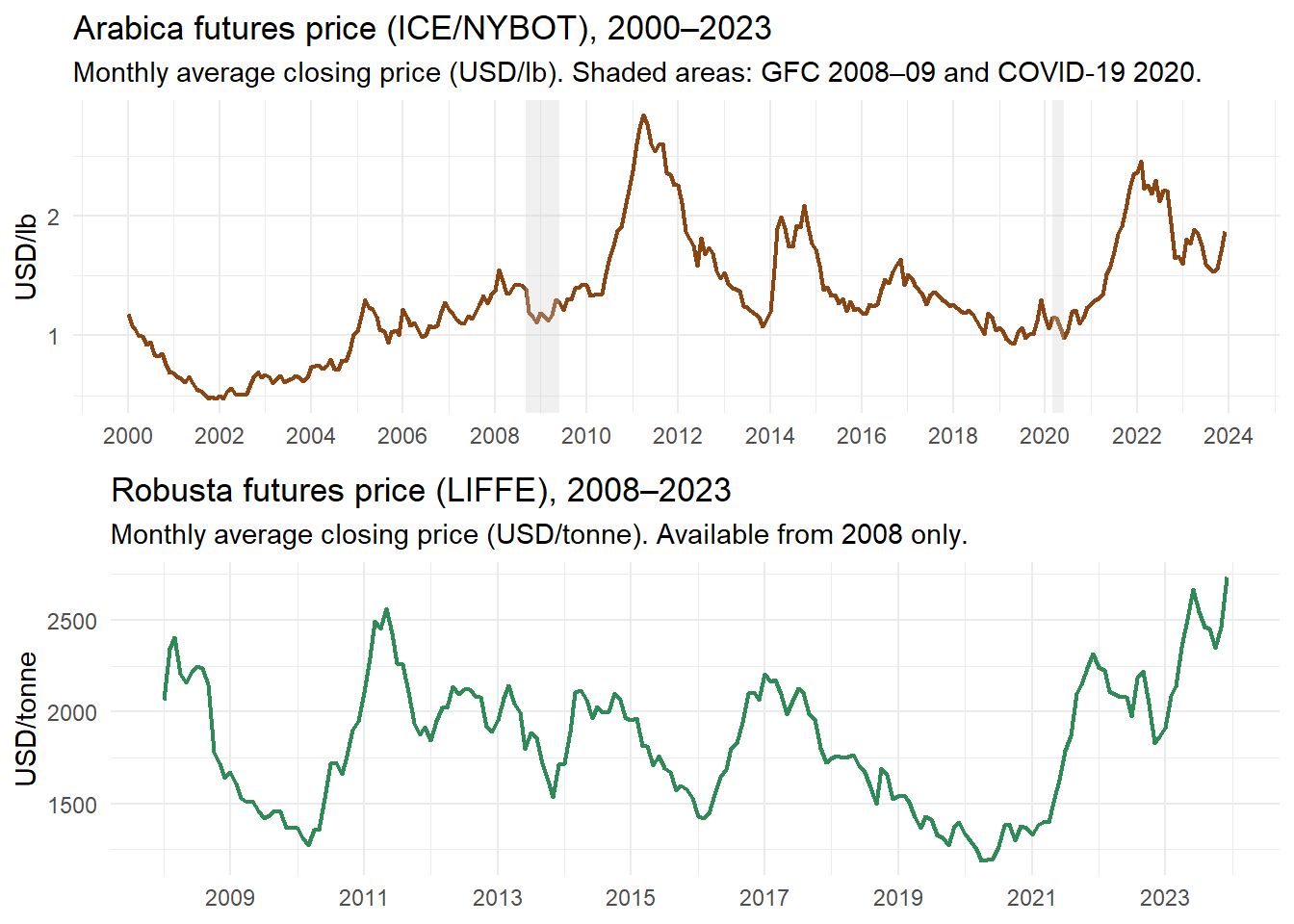
The two dependent variables are the monthly average closing prices of Arabica coffee futures traded on the ICE Futures U.S. exchange (NYBOT, contract code KCc) and Robusta coffee futures traded on the London International Financial Futures Exchange (LIFFE, contract code RCc). Both series are extracted from Refinitiv Eikon via the CEDIF data facility at UNIL, which constitutes the primary source for price data in this study. Arabica and Robusta are treated as two distinct dependent variables and modelled separately throughout the analysis, reflecting their different market structures, consumer bases and price determinants. A combined coffee price index is not constructed, as aggregation would obscure the variety-specific dynamics that this study aims to capture.
Daily closing prices are aggregated to monthly frequency by computing the arithmetic mean of all trading days within each calendar month. This averaging approach is preferred to using the last trading day's price because it is less sensitive to end-of-month volatility spikes associated with contract rollovers, and more representative of the price environment faced by market participants throughout the month.
The use of Refinitiv Eikon as the primary source for futures price data ensures institutional-grade data quality, with prices reflecting actual transaction records from the ICE and LIFFE exchanges rather than aggregated or estimated values from secondary sources.
This chunk reads the four Refinitiv price series — Arabica, Robusta, Cocoa and Sugar — from their raw Excel files and aggregates them from daily to monthly frequency. A single reusable function handles the parsing logic for all four files, which share the same Refinitiv export format. The chunk then builds the time series plots for the two dependent variables.
```{r prix_arabica_robusta, message = FALSE}
# ----------------------------------------------------------
# READING FUNCTION — REFINITIV EXCEL FORMAT
# Refinitiv exports contain metadata rows above the actual
# data. The function locates the header row by searching for
# the string "Exchange Date" in the first column, discards
# everything above it, converts the raw Excel date serial
# numbers to proper R Date objects, and aggregates daily
# closing prices to monthly averages.
#
# Arguments:
#   fichier       : path to the .xlsx file
#   nom_variable  : name to assign to the price column
#                   in the returned data frame
# Returns:
#   A two-column data frame: date (YYYY-MM) and the named
#   monthly average price variable.
# ----------------------------------------------------------

lire_refinitiv <- function(fichier, nom_variable) {

  # Read the raw file without column names (metadata rows present)
  df_raw <- read_excel(fichier, col_names = FALSE)

  # Locate the header row containing "Exchange Date"
  idx_hdr <- which(sapply(df_raw[[1]], function(x)
    identical(as.character(x), "Exchange Date")))
  if (length(idx_hdr) == 0) stop("Header not found in: ", fichier)

  # Retain only the two relevant columns (date and close price)
  # starting from the row immediately after the header
  df_data <- df_raw[(idx_hdr + 1):nrow(df_raw), 1:2]
  colnames(df_data) <- c("date_raw", "close")

  df_data %>%
    mutate(
      # Refinitiv stores dates as Excel serial numbers (days since
      # 1899-12-30). Multiply by 86400 to convert to POSIX seconds.
      date_raw = as.Date(as.POSIXct(as.numeric(date_raw) * 86400,
                                     origin = "1899-12-30", tz = "UTC")),
      close = as.numeric(close)
    ) %>%
    filter(!is.na(date_raw), !is.na(close)) %>%
    arrange(date_raw) %>%
    # Aggregate to monthly frequency: compute the arithmetic mean
    # of all trading days within each calendar month.
    # This is preferred over end-of-month prices as it is less
    # sensitive to contract rollover volatility.
    mutate(date = format(date_raw, "%Y-%m")) %>%
    group_by(date) %>%
    summarise(!!nom_variable := mean(close, na.rm = TRUE), .groups = "drop")
}

# Apply the function to all four Refinitiv price series
arabica  <- lire_refinitiv(FICHIER_ARABICA,  "prix_arabica")
robusta  <- lire_refinitiv(FICHIER_ROBUSTA,  "prix_robusta")
cacao_ny <- lire_refinitiv(FICHIER_CACAO_NY, "prix_cacao")
sucre_11 <- lire_refinitiv(FICHIER_SUCRE_11, "prix_sucre")


# ----------------------------------------------------------
# PLOT DATA — DEPENDENT VARIABLES
# Build a complete monthly date spine covering the full
# analysis period, then left-join the two coffee price
# series. Left-joining preserves all months in the spine,
# so months with no Robusta data (2000-2007) appear as NA
# rather than being silently dropped.
# ----------------------------------------------------------

df_prix <- data.frame(
  date = format(seq(as.Date("2000-01-01"),
                    as.Date("2023-12-01"), by = "month"), "%Y-%m")
) %>%
  left_join(arabica, by = "date") %>%
  left_join(robusta, by = "date") %>%
  mutate(date_fmt = as.Date(paste0(date, "-01")))


# ----------------------------------------------------------
# PLOT 1 — ARABICA FUTURES PRICE (2000-2023)
# Shaded rectangles highlight two major macroeconomic shocks:
# the Global Financial Crisis (Sep 2008 - Jun 2009) and the
# first wave of COVID-19 (Mar - Jun 2020).
# ----------------------------------------------------------

p1 <- ggplot(df_prix, aes(x = date_fmt, y = prix_arabica)) +
  geom_line(color = "#8B4513", linewidth = 0.8) +
  annotate("rect",
           xmin = as.Date("2008-09-01"), xmax = as.Date("2009-06-01"),
           ymin = -Inf, ymax = Inf,
           fill = "grey80", alpha = 0.3) +
  annotate("rect",
           xmin = as.Date("2020-03-01"), xmax = as.Date("2020-06-01"),
           ymin = -Inf, ymax = Inf,
           fill = "grey80", alpha = 0.3) +
  labs(title    = "Arabica futures price (ICE/NYBOT), 2000–2023",
       subtitle = "Monthly average closing price (USD/lb). Shaded areas: GFC 2008–09 and COVID-19 2020.",
       x = NULL, y = "USD/lb") +
  theme_minimal(base_size = 11) +
  scale_x_date(date_breaks = "2 years", date_labels = "%Y")


# ----------------------------------------------------------
# PLOT 2 — ROBUSTA FUTURES PRICE (2008-2023)
# Rows with NA Robusta prices (2000-2007) are excluded before
# plotting to avoid a misleading gap at the left of the axis.
# ----------------------------------------------------------

p2 <- ggplot(filter(df_prix, !is.na(prix_robusta)),
             aes(x = date_fmt, y = prix_robusta)) +
  geom_line(color = "#2E8B57", linewidth = 0.8) +
  labs(title    = "Robusta futures price (LIFFE), 2008–2023",
       subtitle = "Monthly average closing price (USD/tonne). Available from 2008 only.",
       x = NULL, y = "USD/tonne") +
  theme_minimal(base_size = 11) +
  scale_x_date(date_breaks = "2 years", date_labels = "%Y")

gridExtra::grid.arrange(p1, p2, ncol = 1)
```
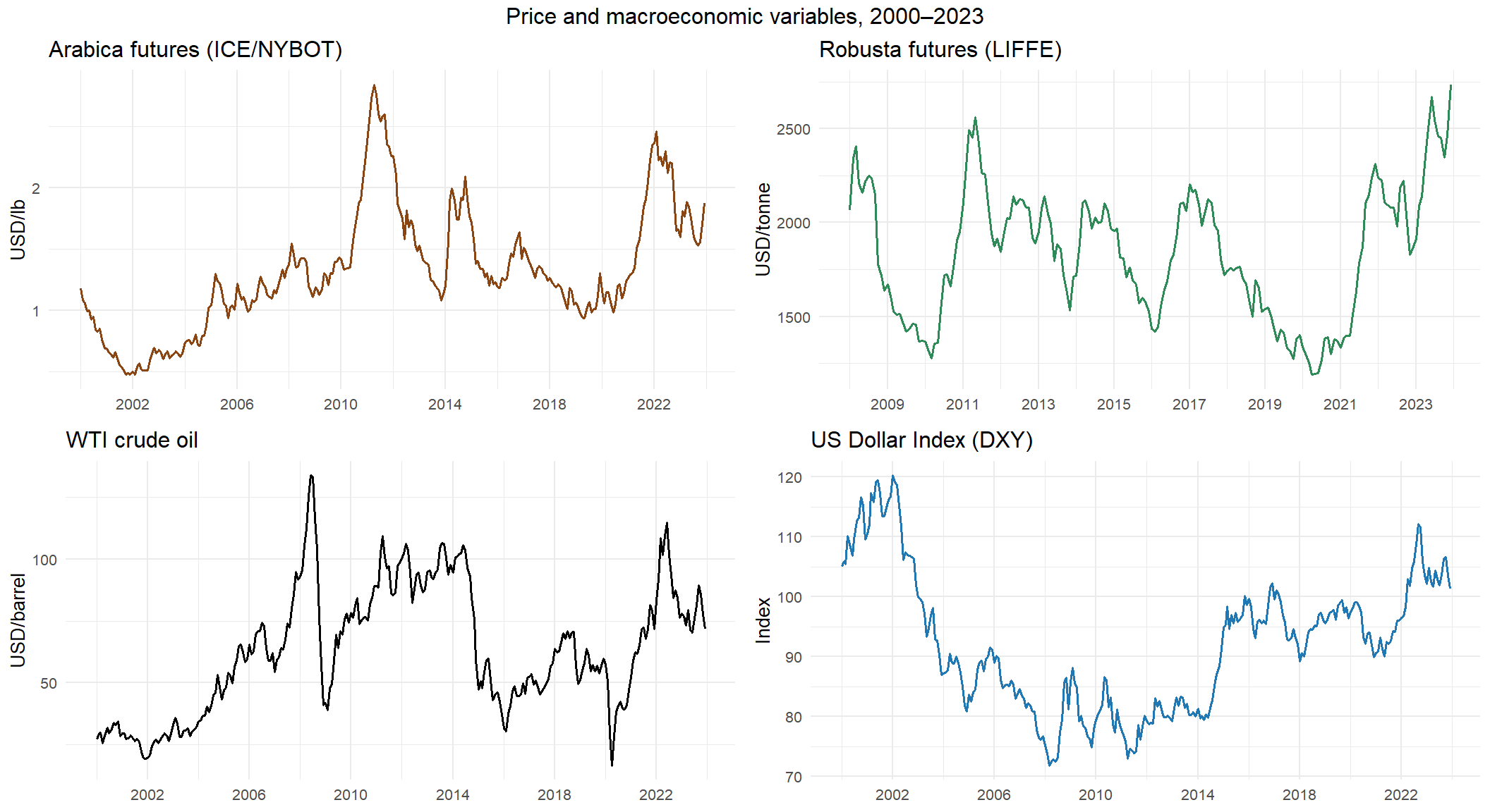
The Arabica price series covers the full 2000–2023 period and exhibits the characteristic volatility of agricultural commodity markets, with a major price spike in 2010–2011 driven by supply shortfalls in Brazil and Colombia, and a renewed surge in 2021–2022 associated with adverse weather conditions and post-pandemic supply chain disruptions. The Robusta series, available from 2008, follows a broadly similar trajectory but at lower absolute price levels, reflecting its use primarily in soluble coffee and blends.
## Market Spillover Variables
Sugar and cocoa prices are included as potential spillover variables. Coffee, sugar and cocoa are all tropical agricultural commodities subject to similar climate shocks and traded on overlapping futures markets. Land substitution between coffee and sugar cultivation in Brazil — the world's largest producer of both — creates a supply-side linkage between the two markets. The Sugar No.11 contract (raw cane sugar, ICE Futures U.S.) and the ICE New York cocoa contract are used, both sourced from Refinitiv via CEDIF and aggregated to monthly frequency using the same procedure as the coffee price series.
## Macroeconomic Variables
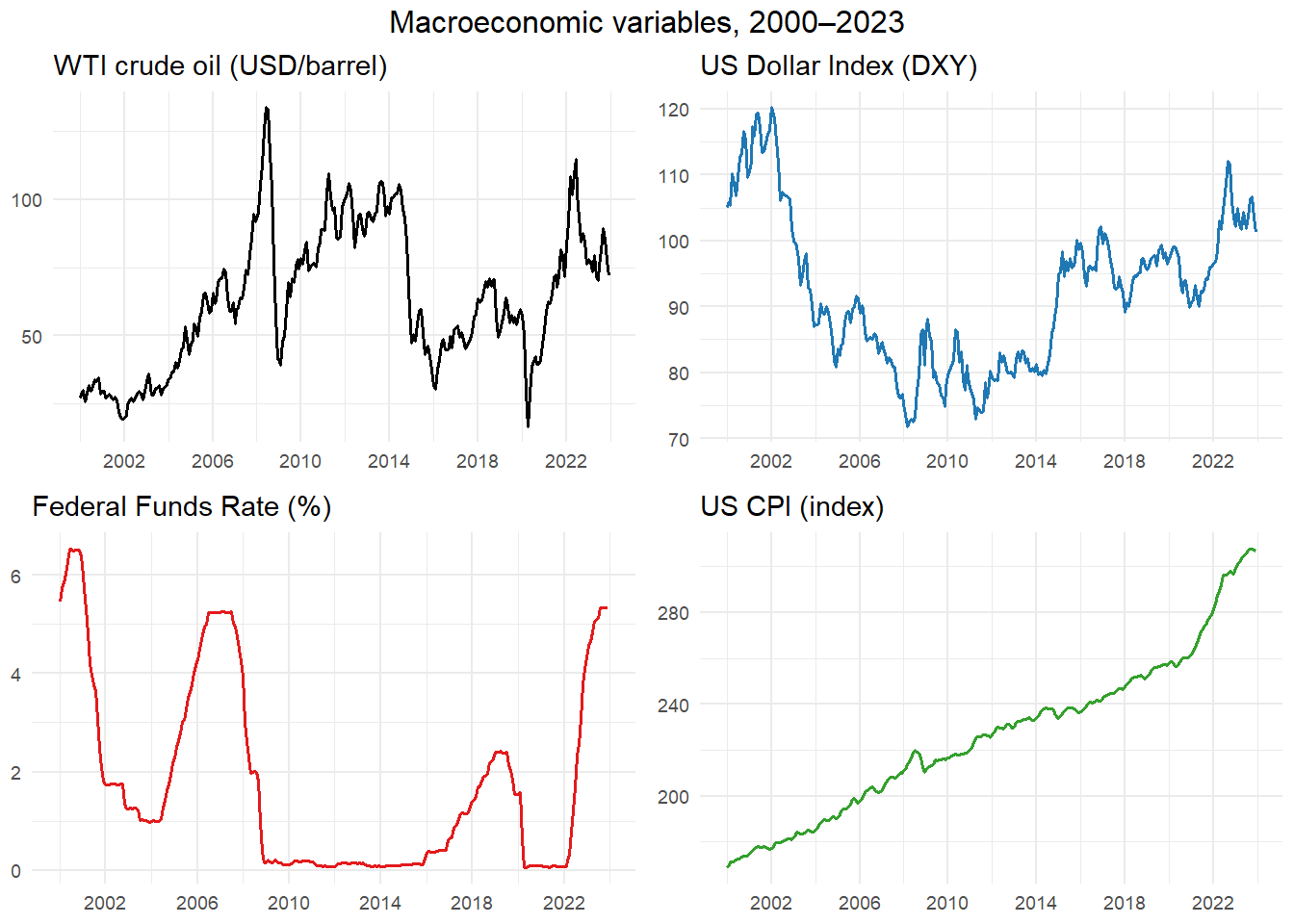
Four macroeconomic variables are included to capture the broader financial and monetary environment that influences commodity prices. All four are sourced from the Federal Reserve Economic Data (FRED) database maintained by the Federal Reserve Bank of St. Louis and are available at monthly frequency.
The WTI crude oil price captures the energy cost dimension of coffee production and transportation, as well as the broad commodity price cycle that tends to co-move across raw materials. The US Dollar Index (DXY), sourced from Investing.com, measures the value of the US dollar against a basket of major currencies; since coffee futures are denominated in US dollars, a stronger dollar tends to depress prices for non-dollar buyers, reducing global demand. The Federal Funds Rate proxies the monetary policy stance of the Federal Reserve, which influences global capital flows, risk appetite and commodity price dynamics. The Consumer Price Index (CPI) captures the general inflation environment.
This chunk reads the four macroeconomic variables from their respective source files and produces a four-panel time series plot. Three series — CPI, WTI and the Federal Funds Rate — are downloaded from FRED and share an identical CSV structure, handled by a single reusable function. The Dollar Index (DXY) requires separate parsing because its Investing.com export uses a different date format and embeds numeric commas in price values.
```{r macro}
# ----------------------------------------------------------
# READING FUNCTION — FRED CSV FORMAT
# FRED exports are two-column CSVs with a date column and
# a value column. The function renames both columns, converts
# the date to YYYY-MM format, and returns a two-column frame
# ready for joining against the monthly date spine.
#
# Arguments:
#   fichier      : path to the .csv file
#   nom_variable : name to assign to the value column
# ----------------------------------------------------------

lire_fred <- function(fichier, nom_variable) {
  df <- read_csv(fichier, show_col_types = FALSE)
  colnames(df) <- c("date_raw", nom_variable)
  df %>%
    mutate(date = format(as.Date(date_raw), "%Y-%m")) %>%
    select(date, all_of(nom_variable))
}

# Apply to the three FRED series
cpi <- lire_fred(FICHIER_CPI, "cpi")
wti <- lire_fred(FICHIER_WTI, "wti")
fed <- lire_fred(FICHIER_FED, "fed_funds_rate")


# ----------------------------------------------------------
# DXY — INVESTING.COM FORMAT (REQUIRES SEPARATE PARSING)
# The Investing.com CSV uses a non-standard date format
# (MM/DD/YYYY), wraps all fields in double quotes, and
# formats numeric values with comma thousands separators
# (e.g. "1,234.56"). Standard read_csv() fails on this
# structure, so the file is read line by line, quotes are
# stripped manually, and commas inside numbers are removed
# before coercing to numeric.
# ----------------------------------------------------------

dxy_lines <- readLines(FICHIER_DXY)

# Remove all double-quote characters from every line
dxy_clean <- gsub('"', '', dxy_lines)

# Re-parse the cleaned text as a standard CSV
dxy_df <- read.csv(text = paste(dxy_clean, collapse = "\n"),
                   stringsAsFactors = FALSE)

dxy <- dxy_df %>%
  select(date_raw = 1, dxy = 2) %>%
  mutate(
    # Remove thousands separator commas before coercing to numeric
    dxy  = as.numeric(gsub(",", "", as.character(dxy))),
    # Convert MM/DD/YYYY date strings to YYYY-MM format
    date = format(as.Date(date_raw, format = "%m/%d/%Y"), "%Y-%m")
  ) %>%
  filter(!is.na(date), !is.na(dxy)) %>%
  arrange(date) %>%
  select(date, dxy)


# ----------------------------------------------------------
# PLOT DATA — MACROECONOMIC VARIABLES
# A complete monthly date spine is built for 2000-2023, then
# all four series are left-joined onto it. Left-joining
# ensures that any months missing from individual series
# appear as NA rather than collapsing the spine.
# ----------------------------------------------------------

df_macro <- data.frame(
  date = format(seq(as.Date("2000-01-01"),
                    as.Date("2023-12-01"), by = "month"), "%Y-%m")
) %>%
  left_join(wti, by = "date") %>%
  left_join(dxy, by = "date") %>%
  left_join(fed, by = "date") %>%
  left_join(cpi, by = "date") %>%
  mutate(date_fmt = as.Date(paste0(date, "-01")))


# ----------------------------------------------------------
# FOUR-PANEL TIME SERIES PLOT
# Each panel uses a distinct color to differentiate the
# series at a glance. No y-axis label is added since the
# panel title already carries the unit information.
# ----------------------------------------------------------

gridExtra::grid.arrange(

  ggplot(df_macro, aes(date_fmt, wti)) +
    geom_line(color = "black", linewidth = 0.6) +
    labs(title = "WTI crude oil (USD/barrel)", x = NULL, y = NULL) +
    theme_minimal(base_size = 9) +
    scale_x_date(date_breaks = "4 years", date_labels = "%Y"),

  ggplot(df_macro, aes(date_fmt, dxy)) +
    geom_line(color = "#1f78b4", linewidth = 0.6) +
    labs(title = "US Dollar Index (DXY)", x = NULL, y = NULL) +
    theme_minimal(base_size = 9) +
    scale_x_date(date_breaks = "4 years", date_labels = "%Y"),

  ggplot(df_macro, aes(date_fmt, fed_funds_rate)) +
    geom_line(color = "#e31a1c", linewidth = 0.6) +
    labs(title = "Federal Funds Rate (%)", x = NULL, y = NULL) +
    theme_minimal(base_size = 9) +
    scale_x_date(date_breaks = "4 years", date_labels = "%Y"),

  ggplot(df_macro, aes(date_fmt, cpi)) +
    geom_line(color = "#33a02c", linewidth = 0.6) +
    labs(title = "US CPI (index)", x = NULL, y = NULL) +
    theme_minimal(base_size = 9) +
    scale_x_date(date_breaks = "4 years", date_labels = "%Y"),

  ncol = 2,
  top  = "Macroeconomic variables, 2000–2023"
)
write.csv(cpi, file.path(PATH_OUTPUT, "cpi.csv"), row.names = FALSE)
write.csv(wti, file.path(PATH_OUTPUT, "wti.csv"), row.names = FALSE)
write.csv(fed, file.path(PATH_OUTPUT, "fed.csv"), row.names = FALSE)
write.csv(dxy, file.path(PATH_OUTPUT, "dxy.csv"), row.names = FALSE)
```
For models estimated at quarterly frequency — specifically those incorporating OECD GDP growth — all monthly macroeconomic variables are aggregated to quarterly frequency by computing the mean of the three constituent months. The OECD quarterly real GDP growth rate (growth rate period-on-period) is sourced from the OECD Data Explorer and covers the 38 OECD member countries, which collectively represent the principal coffee-consuming economies. This variable captures the demand-side dynamics of the global coffee market: when economic activity accelerates in OECD countries, per-capita coffee consumption tends to increase, exerting upward pressure on prices.
## Market Fundamentals: USDA Production, Supply and Distribution
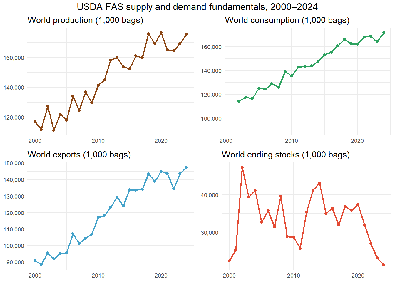
Supply-and-demand fundamentals are sourced from the USDA Foreign Agricultural Service Production, Supply and Distribution (PSD) Online database, which publishes annual crop-year estimates for over 190 countries across all major agricultural commodities. Four variables are retained: world coffee production, world domestic consumption, world exports and world ending stocks. These are aggregated to world totals by summing across all countries for each crop year.
This chunk reads the USDA FAS PSD export file, aggregates country-level data to world totals for the four supply-and-demand variables, and expands the resulting annual series to monthly frequency by repeating each crop-year value across the twelve months of that year. The raw file uses an unusual structure — a single-column CSV embedded inside an Excel file — which requires a two-step parsing approach before standard tidyverse operations can be applied.
```{r usda, message=FALSE, warning=FALSE}
# ----------------------------------------------------------
# STEP 1 — PARSE THE RAW USDA FILE
# The USDA FAS PSD export is structured as an Excel file
# whose first column contains a single long CSV string, with
# the header in row 1 and one data record per subsequent row.
# The file is first read as a raw Excel object, then the
# embedded CSV is reconstructed and parsed properly.
# ----------------------------------------------------------

df_usda_raw <- read_excel(FICHIER_USDA, col_names = FALSE)

# Extract the header string from cell [1,1]
col_name <- as.character(df_usda_raw[1, 1])

# Extract all non-empty data rows from column 1
lignes <- df_usda_raw[-1, 1] %>%
  pull() %>%
  na.omit() %>%
  as.character()

# Reassemble and parse as a standard CSV
df_usda <- read_csv(I(paste(c(col_name, lignes), collapse = "\n")),
                    show_col_types = FALSE)


# ----------------------------------------------------------
# STEP 2 — AGGREGATE TO WORLD TOTALS
# The PSD database contains one row per country per crop year
# per attribute. Summing across all countries yields world
# totals for the four variables of interest.
# Consumption for crop year 2000 is set to NA due to
# incomplete EU reporting in the PSD for that year.
# ----------------------------------------------------------

df_usda_world <- df_usda %>%
  filter(Attribute_Description %in% c("Production", "Domestic Consumption",
                                       "Exports", "Ending Stocks"),
         Market_Year >= 2000, Market_Year <= 2024) %>%
  group_by(Market_Year, Attribute_Description) %>%
  summarise(valeur = sum(Value, na.rm = TRUE), .groups = "drop") %>%
  # Reshape from long to wide: one column per supply-demand variable
  pivot_wider(names_from = Attribute_Description, values_from = valeur) %>%
  rename(annee         = Market_Year,
         production    = Production,
         consommation  = `Domestic Consumption`,
         exportations  = Exports,
         ending_stocks = `Ending Stocks`) %>%
  arrange(annee) %>%
  # Flag year-2000 consumption as missing (incomplete source data)
  mutate(consommation = ifelse(annee == 2000, NA, consommation))


# ----------------------------------------------------------
# STEP 3 — EXPAND TO MONTHLY FREQUENCY
# USDA data are published at annual crop-year frequency.
# Each year's value is repeated across the 12 calendar months
# of that year, reflecting the assumption that market
# participants incorporate annual supply-demand estimates
# into pricing decisions throughout the crop year.
# ----------------------------------------------------------

df_usda_monthly <- df_usda_world %>%
  rowwise() %>%
  do({
    annee <- .$annee
    data.frame(
      date          = format(seq(as.Date(paste0(annee, "-01-01")),
                                 as.Date(paste0(annee, "-12-01")),
                                 by = "month"), "%Y-%m"),
      production    = .$production,
      consommation  = .$consommation,
      exportations  = .$exportations,
      ending_stocks = .$ending_stocks
    )
  }) %>%
  ungroup()


# ----------------------------------------------------------
# STEP 4 — FOUR-PANEL PLOT OF ANNUAL WORLD TOTALS
# The plot uses the annual (non-expanded) data for clarity.
# Each point represents one crop year. Consumption starts
# at 2001 to avoid plotting the documented NA for 2000.
# A minimum y-axis floor of 90,000 is applied to consumption
# to prevent the axis from starting at zero and compressing
# the visible variation in the series.
# ----------------------------------------------------------

df_usda_plot <- df_usda_world %>%
  mutate(date_fmt = as.Date(paste0(annee, "-01-01")))

gridExtra::grid.arrange(

  ggplot(df_usda_plot, aes(date_fmt, production)) +
    geom_line(color = "#8B4513", linewidth = 0.8, na.rm = TRUE) +
    geom_point(size = 1.5, color = "#8B4513", na.rm = TRUE) +
    scale_y_continuous(labels = scales::comma) +
    labs(title = "World production (1,000 bags)", x = NULL, y = NULL) +
    theme_minimal(base_size = 9),

  # Filter out 2000 NA so the consumption chart starts cleanly at 2001
  ggplot(filter(df_usda_plot, !is.na(consommation)),
         aes(date_fmt, consommation)) +
    geom_line(color = "#2ca25f", linewidth = 0.8) +
    geom_point(size = 1.5, color = "#2ca25f") +
    scale_y_continuous(labels = scales::comma, limits = c(90000, NA)) +
    labs(title = "World consumption (1,000 bags)", x = NULL, y = NULL) +
    theme_minimal(base_size = 9),

  ggplot(df_usda_plot, aes(date_fmt, exportations)) +
    geom_line(color = "#43a2ca", linewidth = 0.8, na.rm = TRUE) +
    geom_point(size = 1.5, color = "#43a2ca", na.rm = TRUE) +
    scale_y_continuous(labels = scales::comma) +
    labs(title = "World exports (1,000 bags)", x = NULL, y = NULL) +
    theme_minimal(base_size = 9),

  ggplot(df_usda_plot, aes(date_fmt, ending_stocks)) +
    geom_line(color = "#e34a33", linewidth = 0.8, na.rm = TRUE) +
    geom_point(size = 1.5, color = "#e34a33", na.rm = TRUE) +
    scale_y_continuous(labels = scales::comma) +
    labs(title = "World ending stocks (1,000 bags)", x = NULL, y = NULL) +
    theme_minimal(base_size = 9),

  ncol = 2,
  top  = "USDA FAS supply and demand fundamentals, 2000–2024"
)
```
Since USDA data are published at annual (crop-year) frequency, they are expanded to monthly frequency by repeating each year's value across the 12 calendar months of that year. This approach assumes that market participants incorporate supply-demand fundamentals into their pricing decisions throughout the entire crop year. While the USDA releases monthly updates to its World Agricultural Supply and Demand Estimates (WASDE), the annual PSD figures used here represent end-of-year consolidated estimates. Repeating the annual value across twelve months is a standard simplification when monthly supply-demand data are unavailable.
## Climate Variables
### Selection of Producer Countries
Climate conditions in coffee-producing regions directly affect supply through their impact on cherry development, flowering and yield. Temperature and precipitation are the two primary climatic determinants of coffee production at the agronomy level. Rather than using a single country or global average, this study constructs weighted climate indices that aggregate conditions across the 14 countries that account for the largest share of world coffee production.
The selection of these 14 countries follows a systematic, data-driven criterion: only countries whose average annual share of world coffee production exceeds 1% over the 2000–2024 period are included. This threshold is computed directly from the USDA FAS PSD data used for the supply fundamentals variables, ensuring full consistency between the production weights and the underlying data source. The table below reports the calculated production shares and confirms the selection criterion.
This chunk derives the country selection criterion for the climate indices directly from the USDA PSD data already loaded in the previous chunk. For each crop year, each country's share of world production is computed, and the 25-year average of that share is then calculated across the full 2000–2024 period. Only countries whose average share meets or exceeds the 1% threshold are retained. Using the same USDA source as the fundamentals variables ensures full consistency between the production weights and the underlying data.
```{r selection_pays, echo=TRUE}
# ----------------------------------------------------------
# STEP 1 — COMPUTE ANNUAL PRODUCTION SHARES BY COUNTRY
# For each crop year, world total production is computed
# first as a denominator, then each country's share is
# expressed as a percentage of that total.
# ----------------------------------------------------------

prod_by_country <- df_usda %>%
  filter(Attribute_Description == "Production",
         Market_Year >= 2000, Market_Year <= 2024) %>%
  group_by(Market_Year) %>%
  # Compute world total for the denominator within each year
  mutate(world_total = sum(Value, na.rm = TRUE)) %>%
  ungroup() %>%
  # Each country's share as a percentage of world production
  mutate(share_pct = Value / world_total * 100) %>%

# ----------------------------------------------------------
# STEP 2 — AVERAGE SHARE OVER 2000-2024 AND APPLY THRESHOLD
# Averaging over 25 years smooths out year-to-year production
# fluctuations caused by weather or disease, yielding stable
# structural weights that reflect each country's long-run
# contribution to global supply.
# The 1% threshold is applied to exclude countries whose
# individual contribution is too small to have a meaningful
# impact on the aggregated climate indices.
# ----------------------------------------------------------

  group_by(Country_Name) %>%
  summarise(avg_share = round(mean(share_pct, na.rm = TRUE), 2),
            .groups = "drop") %>%
  arrange(desc(avg_share)) %>%
  filter(avg_share >= 1.0) %>%
  # Correct encoding of Côte d'Ivoire (stored without accent in USDA PSD)
  mutate(Country_Name = recode(Country_Name,
                                "Cote d'Ivoire" = "Côte d'Ivoire"))


# ----------------------------------------------------------
# STEP 3 — DISPLAY THE SELECTION TABLE
# The caption dynamically computes the combined production
# share of the selected countries, confirming that the 14
# retained countries collectively represent ~90.8% of world
# production over the analysis period.
# ----------------------------------------------------------

kable(prod_by_country,
      caption = paste0("Countries with average annual production share ≥ 1%, ",
                       "2000–2024 (USDA FAS PSD). ",
                       "Total: ", round(sum(prod_by_country$avg_share), 1), "%."),
      col.names = c("Country", "Avg. share (%)"),
      booktabs  = TRUE) %>%
  kable_styling(bootstrap_options = c("striped", "hover"),
                font_size = 11, full_width = FALSE)
```
This chunk converts the raw production shares computed in the previous chunk into normalised weights that sum exactly to one. These weights are the core of the climate index construction: every weighted average in the subsequent climate chunks is computed using `POIDS_PRODUCTION`. Two parallel vectors map official country names as they appear in the USDA PSD database to the internal identifiers used in the file lists defined in the setup chunk, ensuring that the correct weight is always matched to the correct file.
```{r poids_production}
# ----------------------------------------------------------
# STEP 1 — DEFINE THE NAME MAPPING BETWEEN USDA AND FILES
# The USDA PSD database uses official English country names,
# while the climate file lists (FICHIERS_PRECIP, FICHIERS_TEMP)
# use shorter internal identifiers without accents, defined
# in the setup chunk. The two vectors below establish the
# one-to-one correspondence between the two naming systems.
# The order in both vectors must be identical.
# ----------------------------------------------------------

pays_retenus  <- c("Brazil", "Vietnam", "Colombia", "Indonesia", "Ethiopia",
                   "India", "Honduras", "Mexico", "Uganda", "Guatemala",
                   "Peru", "Côte d'Ivoire", "Nicaragua", "Costa Rica")

noms_internes <- c("bresil", "vietnam", "colombie", "indonesie", "ethiopie",
                   "inde", "honduras", "mexique", "uganda", "guatemala",
                   "perou", "cote_ivoire", "nicaragua", "costa_rica")


# ----------------------------------------------------------
# STEP 2 — BUILD THE RAW PRODUCTION SHARE VECTOR
# match() looks up each country name from prod_by_country
# in pays_retenus and returns its position, which is then
# used to retrieve the corresponding internal identifier.
# setNames() attaches those identifiers as vector names,
# so that PARTS_PRODUCTION["bresil"] returns Brazil's share.
# ----------------------------------------------------------

PARTS_PRODUCTION <- setNames(
  prod_by_country$avg_share,
  noms_internes[match(prod_by_country$Country_Name, pays_retenus)]
)


# ----------------------------------------------------------
# STEP 3 — NORMALISE TO UNIT SUM (PRODUCTION WEIGHTS)
# Dividing by the total ensures the weights sum exactly to 1,
# as required by the weighted index formula. This normalisation
# step is necessary because the 14 selected countries do not
# collectively account for 100% of world production — the
# remaining ~9% belongs to countries below the 1% threshold.
# ----------------------------------------------------------

POIDS_PRODUCTION <- PARTS_PRODUCTION / sum(PARTS_PRODUCTION)


# ----------------------------------------------------------
# VERIFICATION
# Confirms that all 14 internal names were matched correctly
# and that no NA values were introduced by the name mapping.
# Any NA in the output would indicate a mismatch between
# pays_retenus and the country names in prod_by_country.
# ----------------------------------------------------------

cat("Names of POIDS_PRODUCTION:", names(POIDS_PRODUCTION), "\n")
```
The 14 selected countries collectively account for `r round(sum(prod_by_country$avg_share), 1)`% of world coffee production on average over 2000–2024. Countries falling below the 1% threshold have a negligible and individually undifferentiated impact on global supply, and their inclusion would add noise without improving the explanatory power of the climate indices.
Before constructing variety-specific production weights, the share of Arabica and Robusta production is computed for each of the 14 retained countries directly from the USDA FAS PSD data. The `Arabica Production` and `Robusta Production` attributes are available as separate line items in the raw dataset, allowing the variety split to be calculated empirically rather than assumed from external sources. This ensures full consistency with the data already used for the global production weights. The table below reports the calculated variety shares for each of the 14 countries over the 2000–2024 period.
```{r variety_splits, echo=TRUE}
# ----------------------------------------------------------
# VARIETY SPLITS — ARABICA VS ROBUSTA PER COUNTRY
# The USDA FAS PSD dataset contains separate line items for
# "Arabica Production" and "Robusta Production" per country.
# Summing across 2000-2024 and computing shares yields the
# empirical variety split for each of the 14 retained countries.
# These splits are used downstream to assign each country
# to the correct variety-specific climate index.
# The recode of Cote d'Ivoire is applied BEFORE the filter
# to ensure the country is correctly matched to pays_retenus.
# ----------------------------------------------------------

splits_variete <- df_usda %>%
  filter(Attribute_Description %in% c("Arabica Production",
                                       "Robusta Production"),
         Market_Year >= 2000, Market_Year <= 2024) %>%
  group_by(Country_Name, Attribute_Description) %>%
  summarise(total = sum(Value, na.rm = TRUE), .groups = "drop") %>%
  pivot_wider(names_from  = Attribute_Description,
              values_from = total,
              values_fill = 0) %>%
  rename(arabica = `Arabica Production`,
         robusta = `Robusta Production`) %>%
  mutate(
    Country_Name = recode(Country_Name,
                          "Cote d'Ivoire" = "Côte d'Ivoire"),
    total        = arabica + robusta,
    pct_arabica  = round(arabica / total * 100, 1),
    pct_robusta  = round(robusta / total * 100, 1)
  ) %>%
  filter(Country_Name %in% pays_retenus) %>%
  arrange(desc(total))

kable(splits_variete %>% select(Country_Name, arabica, robusta,
                                 total, pct_arabica, pct_robusta),
      caption   = "Variety splits — Arabica vs Robusta production share per country (2000–2024, USDA FAS PSD)",
      booktabs  = TRUE,
      col.names = c("Country", "Arabica (1000 bags)",
                    "Robusta (1000 bags)", "Total",
                    "% Arabica", "% Robusta")) %>%
  kable_styling(bootstrap_options = c("striped", "hover"),
                font_size = 11, full_width = TRUE)
```
The variety split table confirms the expected production geography of the two coffee varieties. Nine countries produce exclusively or quasi-exclusively Arabica — Colombia, Ethiopia, Honduras, Peru, Costa Rica, Guatemala, Nicaragua and Mexico all report Arabica shares above 90%, and are therefore assigned entirely to the Arabica group. Brazil, the world's largest producer, is the only major country with a significant mixed production, reporting 72.3% Arabica and 27.7% Robusta over the 2000–2024 period. On the Robusta side, Vietnam and Côte d'Ivoire are quasi-pure Robusta producers at 96.8% and 100% respectively, while Indonesia (87.7%), Uganda (80.9%) and India (67.8%) produce predominantly but not exclusively Robusta.
Four countries contribute to both variety-specific indices: Brazil, India, Uganda and Indonesia. For these countries, the production weight assigned to each group is scaled by the empirically computed variety share rather than assumed from external sources. Countries with a variety share above 90% are treated as pure producers and assigned entirely to their dominant group — a simplification justified by the negligible contribution of the minority variety to their total output. This variety-aware weighting scheme ensures that the climate indices used in each model specification reflect conditions in the actual producing zones for that variety, rather than averaging over climatically relevant and irrelevant regions indiscriminately.
The variety-specific production weights are now constructed for each group. For the Arabica group, the nine producing countries are assigned weights proportional to their Arabica production share, adjusted by the empirically computed variety splits for mixed producers. The resulting weights sum to one and reflect the long-run structural contribution of each country to global Arabica supply over 2000–2024.
```{r poids_arabica}
# ----------------------------------------------------------
# VARIETY-SPECIFIC PRODUCTION WEIGHTS — ARABICA GROUP
# Countries assigned to the Arabica group and their variety
# splits (from splits_variete). Countries with >90% Arabica
# share are treated as pure producers (split = 1.0).
# Mixed producers (Brazil, India, Uganda, Indonesia) receive
# their empirically computed Arabica share as a scaling factor.
# ----------------------------------------------------------

# Variety splits for Arabica group
# Pure producers (>90%) get 1.0, mixed producers get actual share
split_arabica <- c(
  bresil      = 0.723,
  colombie    = 1.000,
  ethiopie    = 1.000,
  inde        = 0.322,
  honduras    = 1.000,
  mexique     = 1.000,
  guatemala   = 1.000,
  perou       = 1.000,
  nicaragua   = 1.000,
  costa_rica  = 1.000
)

# Extract raw production shares for Arabica countries
# Uganda, Vietnam, Indonesia, Cote d'Ivoire are excluded
# as they are assigned to the Robusta group
noms_arabica <- names(split_arabica)

PARTS_ARABICA_RAW <- PARTS_PRODUCTION[
  names(PARTS_PRODUCTION) %in% noms_arabica
]

# Apply variety split to adjust for mixed producers
PARTS_ARABICA_ADJ <- PARTS_ARABICA_RAW *
  split_arabica[names(PARTS_ARABICA_RAW)]

# Normalise to unit sum
POIDS_ARABICA <- PARTS_ARABICA_ADJ / sum(PARTS_ARABICA_ADJ,
                                          na.rm = TRUE)

# Display verification table
df_poids_arabica <- data.frame(
  Country     = names(POIDS_ARABICA),
  Raw_share   = round(PARTS_ARABICA_RAW[names(POIDS_ARABICA)], 4),
  Split       = round(split_arabica[names(POIDS_ARABICA)], 3),
  Adj_share   = round(PARTS_ARABICA_ADJ[names(POIDS_ARABICA)], 4),
  Final_weight = round(POIDS_ARABICA, 4)
)

kable(df_poids_arabica,
      caption   = "Arabica production weights — variety-adjusted (2000–2024)",
      booktabs  = TRUE,
      row.names = FALSE,
      col.names = c("Country", "Raw share", "Arabica split",
                    "Adjusted share", "Final weight")) %>%
  kable_styling(bootstrap_options = c("striped", "hover"),
                font_size = 11, full_width = FALSE)
```
The same procedure is applied to the Robusta group. Five countries are assigned to this group — Vietnam, Indonesia, Uganda, Côte d'Ivoire and India — with variety splits applied to the four mixed producers. Vietnam and Côte d'Ivoire are treated as pure Robusta producers given their shares of 96.8% and 100% respectively.
```{r poids_robusta}
# ----------------------------------------------------------
# VARIETY-SPECIFIC PRODUCTION WEIGHTS — ROBUSTA GROUP
# Countries assigned to the Robusta group and their variety
# splits (from splits_variete). Vietnam and Cote d'Ivoire
# are treated as pure producers (split = 1.0).
# Mixed producers (Indonesia, Uganda, India, Brazil) receive
# their empirically computed Robusta share as a scaling factor.
# ----------------------------------------------------------

# Variety splits for Robusta group
split_robusta <- c(
  vietnam     = 1.000,
  indonesie   = 0.877,
  uganda      = 0.809,
  cote_ivoire = 1.000,
  inde        = 0.678,
  bresil      = 0.277
)

# Extract raw production shares for Robusta countries
noms_robusta <- names(split_robusta)

PARTS_ROBUSTA_RAW <- PARTS_PRODUCTION[
  names(PARTS_PRODUCTION) %in% noms_robusta
]

# Apply variety split to adjust for mixed producers
PARTS_ROBUSTA_ADJ <- PARTS_ROBUSTA_RAW *
  split_robusta[names(PARTS_ROBUSTA_RAW)]

# Normalise to unit sum
POIDS_ROBUSTA <- PARTS_ROBUSTA_ADJ / sum(PARTS_ROBUSTA_ADJ,
                                          na.rm = TRUE)

# Display verification table
df_poids_robusta <- data.frame(
  Country      = names(POIDS_ROBUSTA),
  Raw_share    = round(PARTS_ROBUSTA_RAW[names(POIDS_ROBUSTA)], 4),
  Split        = round(split_robusta[names(POIDS_ROBUSTA)], 3),
  Adj_share    = round(PARTS_ROBUSTA_ADJ[names(POIDS_ROBUSTA)], 4),
  Final_weight = round(POIDS_ROBUSTA, 4)
)

kable(df_poids_robusta,
      caption   = "Robusta production weights — variety-adjusted (2000–2024)",
      booktabs  = TRUE,
      row.names = FALSE,
      col.names = c("Country", "Raw share", "Robusta split",
                    "Adjusted share", "Final weight")) %>%
  kable_styling(bootstrap_options = c("striped", "hover"),
                font_size = 11, full_width = FALSE)
```
### Climate Data Source and Spatial Resolution
Temperature and precipitation data are sourced from the World Bank Climate Knowledge Portal (CCKP), which provides access to the ERA5 reanalysis dataset produced by the European Centre for Medium-Range Weather Forecasts (ECMWF). ERA5 offers a spatial resolution of 0.25 degrees (approximately 28 km × 28 km at the equator), which is among the finest resolutions available for global gridded climate datasets covering the full 2000–2023 period.
Data are extracted at the Administrative Division Level 1 (ADM1) — that is, at the province or state level within each country. This sub-national resolution is preferred over country-level averages because coffee cultivation is highly concentrated within specific regions of each country. In Brazil, for instance, production is concentrated in Minas Gerais, São Paulo and Espírito Santo, while the Amazon basin produces virtually none. Using ADM1-level data allows the weighted climate indices to better reflect conditions in the actual producing zones, rather than averaging over climatically diverse national territories.
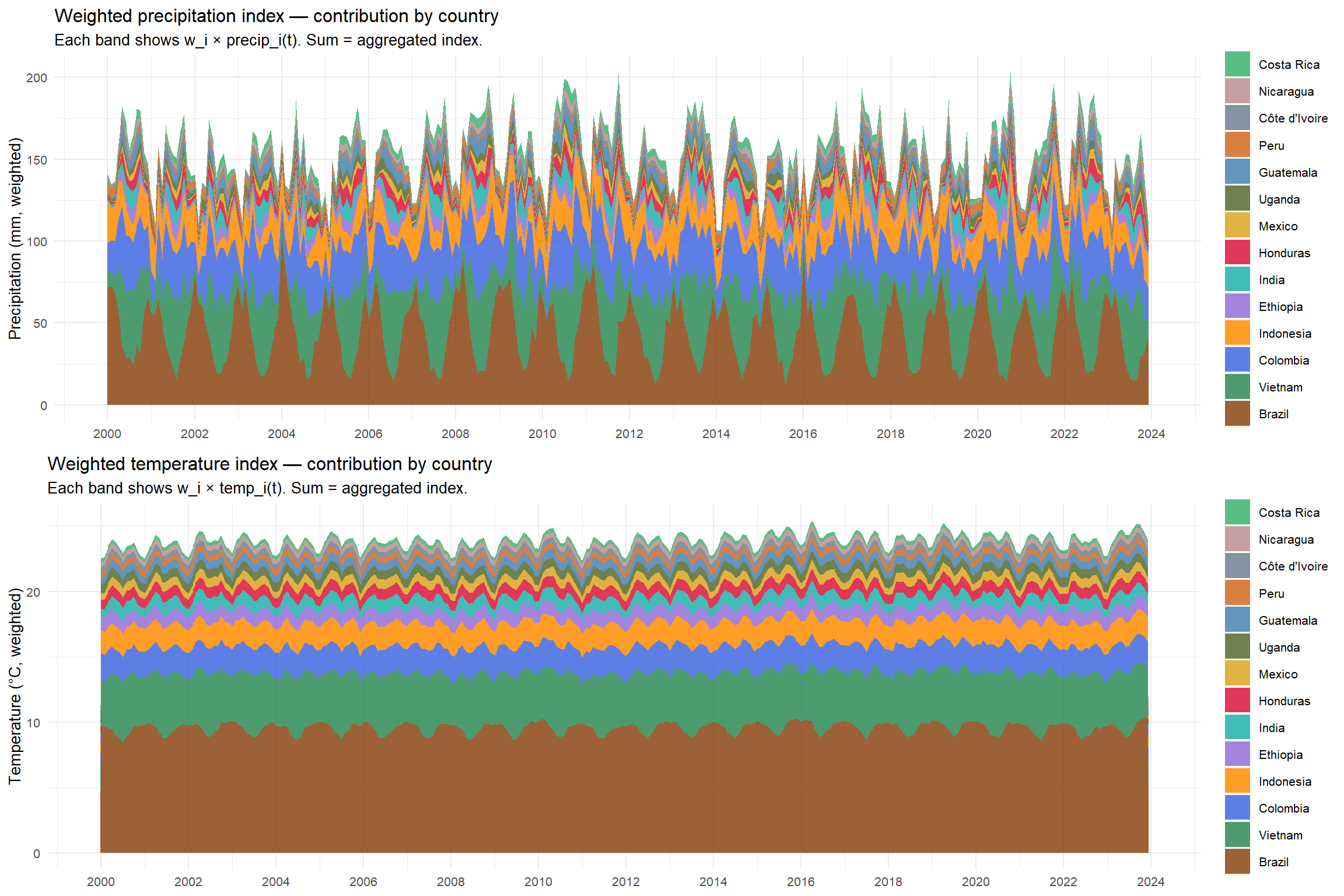
### Construction of the Weighted Climate Indices
For each of the 14 countries, a national monthly average is computed by taking the simple arithmetic mean across all ADM1 regions within the country. The weighted global index is then constructed as follows:
$$\text{Index}(t) = \sum_{i=1}^{14} w_i \cdot X_i(t)$$
where $X_i(t)$ is the national average value of the climate variable (precipitation in mm or temperature in °C) for country $i$ in month $t$, and $w_i$ is the normalised production weight of country $i$ (with $\sum w_i = 1$).
The production weights are held constant at their 2000–2024 averages rather than varying year by year. This fixed-weight approach is adopted to avoid a simultaneity problem: if a climate shock in year $t$ reduces production in a given country, its production share — and therefore its weight in the climate index — would be lower precisely in the year when the shock is most severe. Using time-varying weights would thus attenuate the very signal the index is designed to capture. Fixed weights computed over a long historical average naturally smooth out year-to-year fluctuations in production shares, avoiding the simultaneity bias that would arise from time-varying weights.
This chunk reads the ERA5 precipitation files for all 14 producer countries, computes a national monthly average across ADM1 regions within each country, and then aggregates the 14 national series into a single production-weighted global precipitation index. The reading logic is encapsulated in a reusable function that is applied to all 14 files simultaneously via `mapply()`. The resulting index is saved to disk for reuse in the final dataset assembly chunk.
```{r precipitations, message=FALSE}
# ----------------------------------------------------------
# READING FUNCTION — ERA5 ADM1 CLIMATE FILES
# Each ERA5 file contains one row per administrative region
# (ADM1) and one column per month, with a header row in row 1
# and two metadata columns ("code" and "name") that identify
# the region. The function strips the metadata columns,
# coerces all remaining values to numeric, and computes the
# simple arithmetic mean across all ADM1 regions within the
# country for each month. This yields a single national
# monthly average series per country.
#
# Arguments:
#   fichier   : path to the .xlsx file for one country
#   nom_pays  : internal country identifier (e.g. "bresil")
#   variable  : prefix for the output column ("precip" here)
#
# Returns:
#   A two-column data frame: date (YYYY-MM) and the named
#   national monthly average (e.g. "precip_bresil").
# ----------------------------------------------------------

lire_climat_pays <- function(fichier, nom_pays, variable = "precip") {

  df_raw <- read_excel(fichier, col_names = FALSE)

  # Promote the first row to column names
  colnames(df_raw) <- as.character(df_raw[1, ])
  df_raw <- df_raw[-1, ]

  # Isolate the date columns by excluding the two metadata columns
  cols_dates <- colnames(df_raw)[!colnames(df_raw) %in% c("code", "name")]

  # Coerce all climate value columns to numeric
  df_valeurs <- df_raw[, cols_dates] %>%
    mutate(across(everything(), as.numeric))

  # Average across all ADM1 regions (rows) for each month (column)
  moyennes <- colMeans(df_valeurs, na.rm = TRUE)

  # Return a tidy two-column data frame
  df_pays <- data.frame(date   = names(moyennes),
                        valeur = as.numeric(moyennes),
                        stringsAsFactors = FALSE)
  colnames(df_pays)[2] <- paste0(variable, "_", nom_pays)
  return(df_pays)
}


# ----------------------------------------------------------
# STEP 1 — READ ALL 14 COUNTRY FILES IN PARALLEL
# mapply() applies lire_climat_pays() to all 14 files at
# once, passing the file path and internal country name from
# FICHIERS_PRECIP simultaneously. The result is a named list
# of 14 two-column data frames, one per country.
# ----------------------------------------------------------

liste_precip <- mapply(FUN      = lire_climat_pays,
                       fichier  = FICHIERS_PRECIP,
                       nom_pays = names(FICHIERS_PRECIP),
                       variable = "precip",
                       SIMPLIFY = FALSE)


# ----------------------------------------------------------
# STEP 2 — MERGE INTO A SINGLE WIDE DATA FRAME
# Reduce() applies left_join() sequentially across the list,
# joining each country's series onto a growing wide frame
# keyed by date. The result has one row per month and one
# column per country (14 precipitation columns total).
# The frame is then filtered to the analysis period.
# ----------------------------------------------------------

df_precip_all <- Reduce(function(x, y) left_join(x, y, by = "date"),
                        liste_precip) %>%
  filter(date >= DATE_DEBUT & date <= DATE_FIN) %>%
  arrange(date)


# ----------------------------------------------------------
# STEP 3 — COMPUTE THE PRODUCTION-WEIGHTED INDEX
# For each month, the weighted precipitation index is the
# dot product of the 14 national averages and POIDS_PRODUCTION.
# The column names are constructed to match the weight vector
# names exactly, ensuring the correct weight is applied to
# each country. rowwise() is used because c_across() requires
# operating on one row at a time.
#
# Index formula:  indice_precip(t) = sum_i [ w_i * precip_i(t) ]
# where w_i are the fixed production weights summing to 1.
# ----------------------------------------------------------

cols_pays_precip <- paste0("precip_", names(POIDS_PRODUCTION))

df_precip_all <- df_precip_all %>%
  rowwise() %>%
  mutate(indice_precip = sum(c_across(all_of(cols_pays_precip)) * POIDS_PRODUCTION,
                             na.rm = TRUE)) %>%
  ungroup()


# ----------------------------------------------------------
# STEP 4 — SAVE THE INDEX TO DISK
# Only the date and index columns are retained. The file is
# saved to the output folder and reloaded in the final
# dataset assembly chunk to avoid recomputing from scratch.
# ----------------------------------------------------------

df_indice_precip <- df_precip_all %>% select(date, indice_precip)

write.csv(df_indice_precip,
          file.path(PATH_OUTPUT, "indice_precip_pondere_2000_2023.csv"),
          row.names = FALSE)

write.csv(df_precip_all %>% select(date, starts_with("precip_")),
          file.path(PATH_OUTPUT, "precip_disaggregated_2000_2023.csv"),
          row.names = FALSE)
```
This chunk applies the exact same pipeline as the precipitation chunk to the temperature data. The `lire_climat_pays()` function defined previously is reused without modification — only the input file list, the variable prefix and the output filename change. The resulting production-weighted temperature index is saved to disk alongside the precipitation index.
```{r temperatures, message=FALSE}
# ----------------------------------------------------------
# STEP 1 — READ ALL 14 COUNTRY TEMPERATURE FILES
# Identical logic to the precipitation chunk: mapply() applies
# lire_climat_pays() to all 14 files in FICHIERS_TEMP,
# returning a named list of national monthly average series.
# The variable argument is set to "temp" so that output
# columns are named "temp_bresil", "temp_vietnam", etc.,
# matching the prefix expected when building cols_pays_temp.
# ----------------------------------------------------------

liste_temp <- mapply(FUN      = lire_climat_pays,
                     fichier  = FICHIERS_TEMP,
                     nom_pays = names(FICHIERS_TEMP),
                     variable = "temp",
                     SIMPLIFY = FALSE)


# ----------------------------------------------------------
# STEP 2 — MERGE AND FILTER TO THE ANALYSIS PERIOD
# Same Reduce/left_join pattern as for precipitation, yielding
# a wide frame with one temperature column per country and
# one row per month over 2000-2023.
# ----------------------------------------------------------

df_temp_all <- Reduce(function(x, y) left_join(x, y, by = "date"),
                      liste_temp) %>%
  filter(date >= DATE_DEBUT & date <= DATE_FIN) %>%
  arrange(date)


# ----------------------------------------------------------
# STEP 3 — COMPUTE THE PRODUCTION-WEIGHTED TEMPERATURE INDEX
# The weighted index formula is identical to the precipitation
# case. Column names are prefixed with "temp_" to select the
# correct columns from the wide frame, and POIDS_PRODUCTION
# provides the same fixed weights used throughout.
#
# Index formula:  indice_temp(t) = sum_i [ w_i * temp_i(t) ]
# where w_i are the fixed production weights summing to 1.
# ----------------------------------------------------------

cols_pays_temp <- paste0("temp_", names(POIDS_PRODUCTION))

df_temp_all <- df_temp_all %>%
  rowwise() %>%
  mutate(indice_temp = sum(c_across(all_of(cols_pays_temp)) * POIDS_PRODUCTION,
                           na.rm = TRUE)) %>%
  ungroup()


# ----------------------------------------------------------
# STEP 4 — SAVE THE INDEX TO DISK
# As with precipitation, only the date and index columns are
# retained. The file is reloaded in the final assembly chunk.
# ----------------------------------------------------------

df_indice_temp <- df_temp_all %>% select(date, indice_temp)

write.csv(df_indice_temp,
          file.path(PATH_OUTPUT, "indice_temp_pondere_2000_2023.csv"),
          row.names = FALSE)

write.csv(df_temp_all %>% select(date, starts_with("temp_")),
          file.path(PATH_OUTPUT, "temp_disaggregated_2000_2023.csv"),
          row.names = FALSE)
```
The production-weighted climate indices constructed in the preceding sections aggregate temperature and precipitation conditions across all 14 producer countries regardless of the coffee variety they produce. As established in the variety split analysis, however, the production geographies of Arabica and Robusta are structurally distinct — Arabica is concentrated in Brazil, Colombia and Central America, while Robusta is dominated by Vietnam, Indonesia, Uganda and Côte d'Ivoire. Aggregating climate conditions across both groups in a single index dilutes the variety-specific signal: conditions in Vietnam are irrelevant to Arabica price formation, and conditions in Colombia are irrelevant to Robusta. Two variety-specific climate indices are therefore constructed using the variety-adjusted production weights derived above, one for each coffee group. The pipeline is identical to that used for the global indices — national ADM1 averages are computed and aggregated using the dot product of national values and variety-specific weights — with the difference that only the countries and weights relevant to each variety are included.
```{r indices_climatiques_arabica, message=FALSE}
# ----------------------------------------------------------
# VARIETY-SPECIFIC CLIMATE INDICES — ARABICA GROUP
# The same lire_climat_pays() function is reused without
# modification. Only the file lists and weight vectors change.
# Arabica group: Brazil, Colombia, Ethiopia, India, Honduras,
# Mexico, Guatemala, Peru, Nicaragua, Costa Rica.
# Mixed producers (Brazil, India) contribute their Arabica
# share only via POIDS_ARABICA.
# ----------------------------------------------------------

# STEP 1 — READ PRECIPITATION FILES FOR ARABICA COUNTRIES
FICHIERS_PRECIP_ARA <- FICHIERS_PRECIP[names(POIDS_ARABICA)]

liste_precip_ara <- mapply(FUN      = lire_climat_pays,
                           fichier  = FICHIERS_PRECIP_ARA,
                           nom_pays = names(FICHIERS_PRECIP_ARA),
                           variable = "precip",
                           SIMPLIFY = FALSE)

df_precip_ara <- Reduce(function(x, y) left_join(x, y, by = "date"),
                        liste_precip_ara) %>%
  filter(date >= DATE_DEBUT & date <= DATE_FIN) %>%
  arrange(date)

# STEP 2 — COMPUTE WEIGHTED PRECIPITATION INDEX — ARABICA
cols_precip_ara <- paste0("precip_", names(POIDS_ARABICA))

df_precip_ara <- df_precip_ara %>%
  rowwise() %>%
  mutate(indice_precip_arabica = sum(
    c_across(all_of(cols_precip_ara)) * POIDS_ARABICA,
    na.rm = TRUE)) %>%
  ungroup()

# STEP 3 — READ TEMPERATURE FILES FOR ARABICA COUNTRIES
FICHIERS_TEMP_ARA <- FICHIERS_TEMP[names(POIDS_ARABICA)]

liste_temp_ara <- mapply(FUN      = lire_climat_pays,
                         fichier  = FICHIERS_TEMP_ARA,
                         nom_pays = names(FICHIERS_TEMP_ARA),
                         variable = "temp",
                         SIMPLIFY = FALSE)

df_temp_ara <- Reduce(function(x, y) left_join(x, y, by = "date"),
                      liste_temp_ara) %>%
  filter(date >= DATE_DEBUT & date <= DATE_FIN) %>%
  arrange(date)

# STEP 4 — COMPUTE WEIGHTED TEMPERATURE INDEX — ARABICA
cols_temp_ara <- paste0("temp_", names(POIDS_ARABICA))

df_temp_ara <- df_temp_ara %>%
  rowwise() %>%
  mutate(indice_temp_arabica = sum(
    c_across(all_of(cols_temp_ara)) * POIDS_ARABICA,
    na.rm = TRUE)) %>%
  ungroup()

# STEP 5 — SAVE TO DISK
df_indice_precip_arabica <- df_precip_ara %>%
  select(date, indice_precip_arabica)

df_indice_temp_arabica <- df_temp_ara %>%
  select(date, indice_temp_arabica)

write.csv(df_indice_precip_arabica,
          file.path(PATH_OUTPUT, "indice_precip_arabica_2000_2023.csv"),
          row.names = FALSE)

write.csv(df_indice_temp_arabica,
          file.path(PATH_OUTPUT, "indice_temp_arabica_2000_2023.csv"),
          row.names = FALSE)
```
```{r indices_climatiques_robusta, message=FALSE}
# ----------------------------------------------------------
# VARIETY-SPECIFIC CLIMATE INDICES — ROBUSTA GROUP
# Identical pipeline to the Arabica chunk. Only the file
# lists and weight vectors change.
# Robusta group: Vietnam, Indonesia, Uganda, Cote d'Ivoire,
# India, Brazil.
# Mixed producers (Brazil, Indonesia, Uganda, India) contribute
# their Robusta share only via POIDS_ROBUSTA.
# ----------------------------------------------------------

# STEP 1 — READ PRECIPITATION FILES FOR ROBUSTA COUNTRIES
FICHIERS_PRECIP_ROB <- FICHIERS_PRECIP[names(POIDS_ROBUSTA)]

liste_precip_rob <- mapply(FUN      = lire_climat_pays,
                           fichier  = FICHIERS_PRECIP_ROB,
                           nom_pays = names(FICHIERS_PRECIP_ROB),
                           variable = "precip",
                           SIMPLIFY = FALSE)

df_precip_rob <- Reduce(function(x, y) left_join(x, y, by = "date"),
                        liste_precip_rob) %>%
  filter(date >= DATE_DEBUT & date <= DATE_FIN) %>%
  arrange(date)

# STEP 2 — COMPUTE WEIGHTED PRECIPITATION INDEX — ROBUSTA
cols_precip_rob <- paste0("precip_", names(POIDS_ROBUSTA))

df_precip_rob <- df_precip_rob %>%
  rowwise() %>%
  mutate(indice_precip_robusta = sum(
    c_across(all_of(cols_precip_rob)) * POIDS_ROBUSTA,
    na.rm = TRUE)) %>%
  ungroup()

# STEP 3 — READ TEMPERATURE FILES FOR ROBUSTA COUNTRIES
FICHIERS_TEMP_ROB <- FICHIERS_TEMP[names(POIDS_ROBUSTA)]

liste_temp_rob <- mapply(FUN      = lire_climat_pays,
                         fichier  = FICHIERS_TEMP_ROB,
                         nom_pays = names(FICHIERS_TEMP_ROB),
                         variable = "temp",
                         SIMPLIFY = FALSE)

df_temp_rob <- Reduce(function(x, y) left_join(x, y, by = "date"),
                      liste_temp_rob) %>%
  filter(date >= DATE_DEBUT & date <= DATE_FIN) %>%
  arrange(date)

# STEP 4 — COMPUTE WEIGHTED TEMPERATURE INDEX — ROBUSTA
cols_temp_rob <- paste0("temp_", names(POIDS_ROBUSTA))

df_temp_rob <- df_temp_rob %>%
  rowwise() %>%
  mutate(indice_temp_robusta = sum(
    c_across(all_of(cols_temp_rob)) * POIDS_ROBUSTA,
    na.rm = TRUE)) %>%
  ungroup()

# STEP 5 — SAVE TO DISK
df_indice_precip_robusta <- df_precip_rob %>%
  select(date, indice_precip_robusta)

df_indice_temp_robusta <- df_temp_rob %>%
  select(date, indice_temp_robusta)

write.csv(df_indice_precip_robusta,
          file.path(PATH_OUTPUT, "indice_precip_robusta_2000_2023.csv"),
          row.names = FALSE)

write.csv(df_indice_temp_robusta,
          file.path(PATH_OUTPUT, "indice_temp_robusta_2000_2023.csv"),
          row.names = FALSE)
```
The same variety-specific logic applied to the climate indices is now extended to the supply-and-demand fundamentals. Rather than using world totals for production, consumption, exports and ending stocks, two variety-specific aggregates are constructed by summing across the countries assigned to each group, weighted by their variety split. This ensures that the fundamentals used in the Arabica models reflect conditions in Arabica-producing countries only, and vice versa for Robusta.
```{r fondamentaux_arabica, message=FALSE, warning=FALSE}
# ----------------------------------------------------------
# VARIETY-SPECIFIC FUNDAMENTALS — ARABICA GROUP
# Production, consumption, exports and ending stocks are
# aggregated across Arabica-producing countries only.
# Mixed producers (Brazil, India, Uganda, Indonesia) contribute
# their Arabica share only, applied to their country-level
# fundamentals before summing to group totals.
# ----------------------------------------------------------

# Arabica countries with their variety splits
arabica_splits_df <- data.frame(
  Country_Name = c("Brazil", "Colombia", "Ethiopia", "India",
                   "Honduras", "Mexico", "Guatemala", "Peru",
                   "Nicaragua", "Costa Rica"),
  split = c(0.723, 1.000, 1.000, 0.322,
            1.000, 1.000, 1.000, 1.000,
            1.000, 1.000),
  stringsAsFactors = FALSE
)

# Apply variety split to fundamentals and aggregate
df_usda_arabica <- df_usda %>%
  filter(Attribute_Description %in% c("Production",
                                       "Domestic Consumption",
                                       "Exports",
                                       "Ending Stocks"),
         Market_Year >= 2000, Market_Year <= 2024) %>%
  # Recode Cote d'Ivoire before join
  mutate(Country_Name = recode(Country_Name,
                                "Cote d'Ivoire" = "Côte d'Ivoire")) %>%
  # Keep only Arabica countries
  inner_join(arabica_splits_df, by = "Country_Name") %>%
  # Apply variety split to each country's value
  mutate(Value_adj = Value * split) %>%
  # Sum across countries for each year and attribute
  group_by(Market_Year, Attribute_Description) %>%
  summarise(valeur = sum(Value_adj, na.rm = TRUE), .groups = "drop") %>%
  pivot_wider(names_from = Attribute_Description,
              values_from = valeur) %>%
  rename(annee                  = Market_Year,
         production_ara         = Production,
         consommation_ara       = `Domestic Consumption`,
         exportations_ara       = Exports,
         ending_stocks_ara      = `Ending Stocks`) %>%
  arrange(annee) %>%
  mutate(consommation_ara = ifelse(annee == 2000, NA, consommation_ara))

# Expand to monthly frequency
df_usda_arabica_monthly <- df_usda_arabica %>%
  rowwise() %>%
  do({
    annee <- .$annee
    data.frame(
      date             = format(seq(as.Date(paste0(annee, "-01-01")),
                                   as.Date(paste0(annee, "-12-01")),
                                   by = "month"), "%Y-%m"),
      production_ara   = .$production_ara,
      consommation_ara = .$consommation_ara,
      exportations_ara = .$exportations_ara,
      ending_stocks_ara = .$ending_stocks_ara
    )
  }) %>%
  ungroup()

write.csv(df_usda_arabica_monthly,
          file.path(PATH_OUTPUT, "fondamentaux_arabica_2000_2023.csv"),
          row.names = FALSE)
```
```{r fondamentaux_robusta, message=FALSE, warning=FALSE}
# ----------------------------------------------------------
# VARIETY-SPECIFIC FUNDAMENTALS — ROBUSTA GROUP
# Identical pipeline to the Arabica chunk.
# Robusta countries: Vietnam, Indonesia, Uganda, Cote d'Ivoire,
# India, Brazil — each with their empirical Robusta split.
# ----------------------------------------------------------

# Robusta countries with their variety splits
robusta_splits_df <- data.frame(
  Country_Name = c("Brazil", "Vietnam", "Indonesia", "India",
                   "Uganda", "Cote d'Ivoire"),
  split = c(0.277, 1.000, 0.877, 0.678,
            0.809, 1.000),
  stringsAsFactors = FALSE
)

# Apply variety split to fundamentals and aggregate
df_usda_robusta <- df_usda %>%
  filter(Attribute_Description %in% c("Production",
                                       "Domestic Consumption",
                                       "Exports",
                                       "Ending Stocks"),
         Market_Year >= 2000, Market_Year <= 2024) %>%
  # Keep original Cote d'Ivoire spelling for join
  inner_join(robusta_splits_df, by = "Country_Name") %>%
  # Apply variety split to each country's value
  mutate(Value_adj = Value * split) %>%
  # Sum across countries for each year and attribute
  group_by(Market_Year, Attribute_Description) %>%
  summarise(valeur = sum(Value_adj, na.rm = TRUE), .groups = "drop") %>%
  pivot_wider(names_from = Attribute_Description,
              values_from = valeur) %>%
  rename(annee                  = Market_Year,
         production_rob         = Production,
         consommation_rob       = `Domestic Consumption`,
         exportations_rob       = Exports,
         ending_stocks_rob      = `Ending Stocks`) %>%
  arrange(annee) %>%
  mutate(consommation_rob = ifelse(annee == 2000, NA, consommation_rob))

# Expand to monthly frequency
df_usda_robusta_monthly <- df_usda_robusta %>%
  rowwise() %>%
  do({
    annee <- .$annee
    data.frame(
      date              = format(seq(as.Date(paste0(annee, "-01-01")),
                                    as.Date(paste0(annee, "-12-01")),
                                    by = "month"), "%Y-%m"),
      production_rob    = .$production_rob,
      consommation_rob  = .$consommation_rob,
      exportations_rob  = .$exportations_rob,
      ending_stocks_rob = .$ending_stocks_rob
    )
  }) %>%
  ungroup()

write.csv(df_usda_robusta_monthly,
          file.path(PATH_OUTPUT, "fondamentaux_robusta_2000_2023.csv"),
          row.names = FALSE)
```
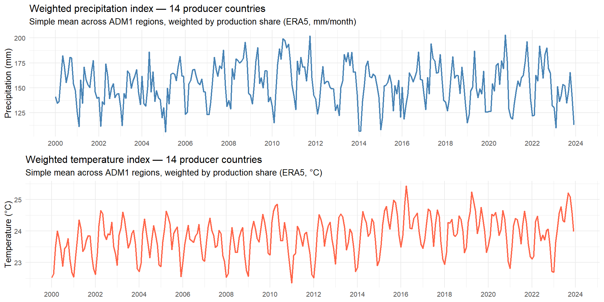
This chunk joins the two climate indices into a single plotting frame and produces a two-panel time series chart for visual inspection. The plot serves as a first diagnostic check on the indices: it allows verifying that the seasonal patterns, trend behaviour and known climate episodes visible in the raw data are correctly reflected in the aggregated series before they enter the modelling pipeline.
```{r plot_climat, fig.width=10, fig.height=5}
# ----------------------------------------------------------
# BUILD THE PLOTTING FRAME
# The two index series are joined on date and a proper Date
# column is added for ggplot's date scale. Both indices are
# already filtered to 2000-2023 from the previous chunks,
# so no further filtering is needed here.
# ----------------------------------------------------------
df_clim_plot <- df_indice_precip %>%
left_join(df_indice_temp, by = "date") %>%
mutate(date_fmt = as.Date(paste0(date, "-01")))
# ----------------------------------------------------------
# TWO-PANEL CLIMATE INDEX PLOT
# Panel 1 — Precipitation index (mm/month)
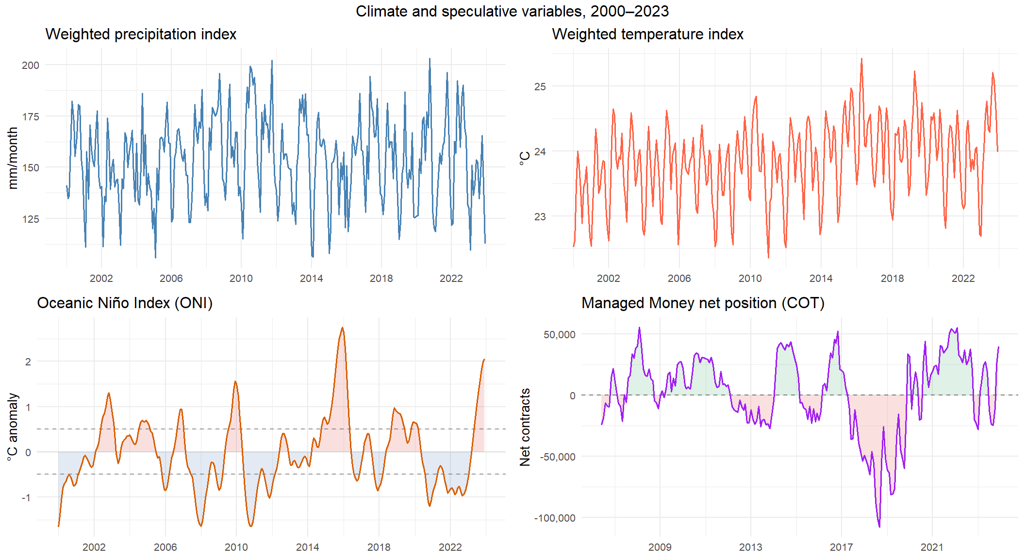
# A strong seasonal cycle is expected and confirms that the
# ADM1 averaging and weighting steps preserved the seasonal
# signal present in the raw country-level data.
#
# Panel 2 — Temperature index (°C)
# A gradual upward trend over the period is consistent with
# documented warming in tropical producing regions. If
# confirmed by the stationarity tests below, this trend
# implies that the temperature series will require first-
# differencing before entering the econometric models.
# ----------------------------------------------------------
gridExtra::grid.arrange(
ggplot(df_clim_plot, aes(date_fmt, indice_precip)) +
geom_line(color = "steelblue", linewidth = 0.8) +
labs(title = "Weighted precipitation index — 14 producer countries",
subtitle = "Simple mean across ADM1 regions, weighted by production share (ERA5, mm/month)",
x = NULL, y = "Precipitation (mm)") +
theme_minimal(base_size = 10) +
scale_x_date(date_breaks = "2 years", date_labels = "%Y"),
ggplot(df_clim_plot, aes(date_fmt, indice_temp)) +
geom_line(color = "tomato", linewidth = 0.8) +
labs(title = "Weighted temperature index — 14 producer countries",
subtitle = "Simple mean across ADM1 regions, weighted by production share (ERA5, °C)",
x = NULL, y = "Temperature (°C)") +
theme_minimal(base_size = 10) +
scale_x_date(date_breaks = "2 years", date_labels = "%Y"),
ncol = 1
)
```
The precipitation index displays a strong seasonal pattern throughout the 2000–2023 period, with no discernible long-term trend, consistent with expectations for a stationary series. Notable dry episodes are visible around 2005–2006 and 2013–2014, corresponding to documented drought periods in Brazil. The temperature index also exhibits seasonal fluctuations but reveals a gradual upward trend over the period, rising from approximately 23°C in 2000 to peaks above 25°C in recent years. This warming pattern is consistent with global climate change trends in tropical producing regions and suggests that the temperature series may be non-stationary in levels — a hypothesis that will be formally tested in the stationarity analysis below.
### Disaggregated Climate Analysis
This section disaggregates the two production-weighted climate indices to show the individual contribution of each of the 14 producer countries. Two complementary visualisations are produced: a stacked area chart showing how each country's weighted contribution evolves over time, and an anomaly heatmap identifying which countries experienced the most significant climate deviations from their long-run averages. Together these plots provide the visual basis for understanding the country-level heterogeneity that the aggregated indices summarise.
```{r climate_contributions, message=FALSE, fig.width=12, fig.height=8}
# ----------------------------------------------------------
# STEP 1 — COMPUTE WEIGHTED CONTRIBUTIONS PER COUNTRY
# For each month t and country i, the contribution to the
# global index is w_i * X_i(t). These contributions sum to
# the aggregated index value at each point in time.
# The data is reshaped from wide to long format for ggplot.
# ----------------------------------------------------------

# Country display names for the legend (same order as POIDS_PRODUCTION)
noms_affichage <- c(
  "bresil"      = "Brazil",
  "vietnam"     = "Vietnam",
  "colombie"    = "Colombia",
  "indonesie"   = "Indonesia",
  "ethiopie"    = "Ethiopia",
  "inde"        = "India",
  "honduras"    = "Honduras",
  "mexique"     = "Mexico",
  "uganda"      = "Uganda",
  "guatemala"   = "Guatemala",
  "perou"       = "Peru",
  "cote_ivoire" = "Côte d'Ivoire",
  "nicaragua"   = "Nicaragua",
  "costa_rica"  = "Costa Rica"
)

# --- PRECIPITATION CONTRIBUTIONS ---
cols_precip <- paste0("precip_", names(POIDS_PRODUCTION))

df_contrib_precip <- df_precip_all %>%
  filter(date >= DATE_DEBUT & date <= DATE_FIN) %>%
  select(date, all_of(cols_precip)) %>%
  # Multiply each country column by its production weight
  mutate(across(all_of(cols_precip),
                ~ .x * POIDS_PRODUCTION[sub("precip_", "", cur_column())])) %>%
  pivot_longer(cols = all_of(cols_precip),
               names_to  = "pays",
               values_to = "contribution") %>%
  mutate(
    pays     = sub("precip_", "", pays),
    pays     = recode(pays, !!!noms_affichage),
    date_fmt = as.Date(paste0(date, "-01")),
    # Order countries by production weight (largest at bottom)
    pays = factor(pays, levels = rev(noms_affichage[names(POIDS_PRODUCTION)]))
  )

# --- TEMPERATURE CONTRIBUTIONS ---
cols_temp <- paste0("temp_", names(POIDS_PRODUCTION))

df_contrib_temp <- df_temp_all %>%
  filter(date >= DATE_DEBUT & date <= DATE_FIN) %>%
  select(date, all_of(cols_temp)) %>%
  mutate(across(all_of(cols_temp),
                ~ .x * POIDS_PRODUCTION[sub("temp_", "", cur_column())])) %>%
  pivot_longer(cols = all_of(cols_temp),
               names_to  = "pays",
               values_to = "contribution") %>%
  mutate(
    pays     = sub("temp_", "", pays),
    pays     = recode(pays, !!!noms_affichage),
    date_fmt = as.Date(paste0(date, "-01")),
    pays = factor(pays, levels = rev(noms_affichage[names(POIDS_PRODUCTION)]))
  )

# Colour palette — 14 distinct colours
palette_pays <- c(
  "Brazil"        = "#8B4513", "Vietnam"      = "#2E8B57",
  "Colombia"      = "#4169E1", "Indonesia"    = "#FF8C00",
  "Ethiopia"      = "#9370DB", "India"        = "#20B2AA",
  "Honduras"      = "#DC143C", "Mexico"       = "#DAA520",
  "Uganda"        = "#556B2F", "Guatemala"    = "#4682B4",
  "Peru"          = "#D2691E", "Côte d'Ivoire"= "#708090",
  "Nicaragua"     = "#BC8F8F", "Costa Rica"   = "#3CB371"
)

# --- PLOT 1 — PRECIPITATION STACKED AREA ---
p_stack_precip <- ggplot(df_contrib_precip,
                         aes(x = date_fmt, y = contribution,
                             fill = pays)) +
  geom_area(position = "stack", alpha = 0.85) +
  scale_fill_manual(values = palette_pays) +
  labs(title    = "Weighted precipitation index — contribution by country",
       subtitle = "Each band shows w_i × precip_i(t). Sum = aggregated index.",
       x = NULL, y = "Precipitation (mm, weighted)",
       fill = NULL) +
  theme_minimal(base_size = 10) +
  scale_x_date(date_breaks = "2 years", date_labels = "%Y") +
  theme(legend.position = "right",
        legend.text     = element_text(size = 8))

# --- PLOT 2 — TEMPERATURE STACKED AREA ---
p_stack_temp <- ggplot(df_contrib_temp,
                       aes(x = date_fmt, y = contribution,
                           fill = pays)) +
  geom_area(position = "stack", alpha = 0.85) +
  scale_fill_manual(values = palette_pays) +
  labs(title    = "Weighted temperature index — contribution by country",
       subtitle = "Each band shows w_i × temp_i(t). Sum = aggregated index.",
       x = NULL, y = "Temperature (°C, weighted)",
       fill = NULL) +
  theme_minimal(base_size = 10) +
  scale_x_date(date_breaks = "2 years", date_labels = "%Y") +
  theme(legend.position = "right",
        legend.text     = element_text(size = 8))

gridExtra::grid.arrange(p_stack_precip, p_stack_temp, ncol = 1)
```
The stacked area charts decompose the two production-weighted climate indices into their country-level contributions, revealing the structural dominance of a small number of producers in shaping the global climate signal.
For precipitation, Brazil accounts for the largest single contribution throughout the entire 2000–2023 period, reflecting both its dominant production weight (approximately 35%) and its high absolute rainfall levels. Vietnam and Colombia form the next tier, together with Indonesia, whose contribution is particularly visible during the wet season peaks. The remaining ten countries collectively occupy the upper portion of the stack but individually contribute narrow bands, confirming that the precipitation index is effectively driven by the top four producers. The strong seasonal oscillation visible across the full stack is consistent with the monsoon and dry season cycles of the tropical producing regions. Notable dips in the Brazilian band around 2005 and 2021 correspond to documented drought episodes in Minas Gerais that triggered significant supply shortfalls and upward price pressure.
For temperature, the structure is markedly more stable. Brazil again dominates the bottom band, but the contributions of all 14 countries are more uniform in relative terms — reflecting the fact that temperature varies less across producing regions than precipitation. The gradual upward drift of the total stack height over the period, most visible from 2015 onward, is the disaggregated counterpart of the warming trend identified in the aggregated temperature index and confirms that it is a broad-based phenomenon affecting multiple producing countries rather than a single-country artefact.
```{r climate_anomalies, message=FALSE, fig.width=12, fig.height=7}
# ----------------------------------------------------------
# STEP 2 — ANOMALY HEATMAP
# For each country and each month, the anomaly is defined as
# the deviation from that country's long-run monthly mean
# over 2000-2023. Standardising by the country's own mean
# puts all countries on a comparable scale regardless of
# their absolute climate levels.
# ----------------------------------------------------------

# --- PRECIPITATION ANOMALIES ---
df_anom_precip <- df_precip_all %>%
  filter(date >= DATE_DEBUT & date <= DATE_FIN) %>%
  select(date, all_of(cols_precip)) %>%
  pivot_longer(cols = all_of(cols_precip),
               names_to  = "pays",
               values_to = "valeur") %>%
  mutate(pays = sub("precip_", "", pays)) %>%
  group_by(pays) %>%
  # Compute anomaly as deviation from country long-run mean
  mutate(anomalie = valeur - mean(valeur, na.rm = TRUE)) %>%
  ungroup() %>%
  mutate(
    pays     = recode(pays, !!!noms_affichage),
    date_fmt = as.Date(paste0(date, "-01")),
    # Order by production weight (most important at top)
    pays = factor(pays,
                  levels = noms_affichage[names(POIDS_PRODUCTION)])
  )

# --- TEMPERATURE ANOMALIES ---
df_anom_temp <- df_temp_all %>%
  filter(date >= DATE_DEBUT & date <= DATE_FIN) %>%
  select(date, all_of(cols_temp)) %>%
  pivot_longer(cols = all_of(cols_temp),
               names_to  = "pays",
               values_to = "valeur") %>%
  mutate(pays = sub("temp_", "", pays)) %>%
  group_by(pays) %>%
  mutate(anomalie = valeur - mean(valeur, na.rm = TRUE)) %>%
  ungroup() %>%
  mutate(
    pays     = recode(pays, !!!noms_affichage),
    date_fmt = as.Date(paste0(date, "-01")),
    pays = factor(pays,
                  levels = noms_affichage[names(POIDS_PRODUCTION)])
  )

# --- HEATMAP — PRECIPITATION ---
p_heatmap_precip <- ggplot(df_anom_precip,
                           aes(x = date_fmt, y = pays,
                               fill = anomalie)) +
  geom_tile() +
  scale_fill_gradient2(low = "#d73027", mid = "white", high = "#4575b4",
                       midpoint = 0,
                       name = "Anomaly\n(mm)") +
  labs(title    = "Precipitation anomalies by country — 2000–2023",
       subtitle = "Deviation from each country's 2000–2023 monthly mean. Blue = wetter than average, Red = drier.",
       x = NULL, y = NULL) +
  theme_minimal(base_size = 10) +
  scale_x_date(date_breaks = "2 years", date_labels = "%Y") +
  theme(axis.text.y = element_text(size = 9),
        legend.position = "right")

# --- HEATMAP — TEMPERATURE ---
p_heatmap_temp <- ggplot(df_anom_temp,
                         aes(x = date_fmt, y = pays,
                             fill = anomalie)) +
  geom_tile() +
  scale_fill_gradient2(low = "#4575b4", mid = "white", high = "#d73027",
                       midpoint = 0,
                       name = "Anomaly\n(°C)") +
  labs(title    = "Temperature anomalies by country — 2000–2023",
       subtitle = "Deviation from each country's 2000–2023 monthly mean. Red = warmer than average, Blue = cooler.",
       x = NULL, y = NULL) +
  theme_minimal(base_size = 10) +
  scale_x_date(date_breaks = "2 years", date_labels = "%Y") +
  theme(axis.text.y = element_text(size = 9),
        legend.position = "right")

gridExtra::grid.arrange(p_heatmap_precip, p_heatmap_temp, ncol = 1)
```
The anomaly heatmaps provide a complementary view by highlighting episodes of abnormal climate conditions at the country level, abstracting from seasonal patterns and absolute levels.
For precipitation, the most striking feature is the heterogeneity of anomaly patterns across countries — wet and dry episodes do not affect all producers simultaneously, which is consistent with the documented asymmetric effects of ENSO on different producing regions. Brazil shows a pronounced negative anomaly (red) around 2021, corresponding to the severe drought in Minas Gerais that contributed to the Arabica price spike of that year. Colombia displays a persistent positive anomaly (blue) during 2010–2011, consistent with the La Niña episode of that period which brought excess rainfall and leaf rust outbreaks to Colombian growing regions. Vietnam and Indonesia show alternating wet and dry episodes broadly aligned with ENSO cycles, while the smaller Central American producers — Honduras, Guatemala, Nicaragua — display high-frequency oscillations that partly reflect their more localised rainfall patterns.
For temperature, the picture is notably different. India stands out with the highest anomaly amplitude of any country — large alternating red and blue blocks throughout the period — suggesting that Indian growing regions experience more pronounced temperature swings than other producers. Brazil and Vietnam both show a gradual drift toward positive anomalies (warmer than average) from approximately 2015 onward, which is consistent with the upward trend visible in the aggregated temperature index and reinforces the conclusion that the warming signal is structural rather than cyclical. Colombia and Indonesia, by contrast, show more balanced anomaly distributions with no clear directional trend, suggesting that their temperature environments have been more stable over the analysis period.
Taken together, the two heatmaps confirm that climate shocks are geographically heterogeneous and that aggregating to a single global index necessarily smooths over country-specific episodes. This heterogeneity motivates the robustness check conducted in the Results section, which tests whether retaining the disaggregated national series improves predictive accuracy relative to the aggregated indices.
## Oceanic Niño Index (ONI)
The Oceanic Niño Index (ONI) is the standard measure of the El Niño–Southern Oscillation (ENSO) phenomenon published by the National Oceanic and Atmospheric Administration (NOAA). It measures the three-month running average of sea surface temperature anomalies in the Niño 3.4 region of the central equatorial Pacific Ocean (5°N–5°S, 120°–170°W), expressed as a departure from a 30-year climatological baseline updated every five years.
The ENSO cycle is one of the most extensively documented climate drivers of coffee price volatility. El Niño episodes — defined as ONI values above +0.5°C sustained for at least five consecutive months — are associated with severe droughts in Brazil and Colombia, reducing production and exerting upward pressure on prices. La Niña episodes (ONI below −0.5°C) bring excessive rainfall to parts of Central America and Southeast Asia, increasing the risk of fungal diseases such as coffee leaf rust.
The variable retained is the ANOM column (temperature anomaly in °C), rather than the TOTAL column (absolute sea surface temperature). The anomaly captures the deviation from normal conditions and is therefore the operationally relevant measure for assessing El Niño or La Niña strength.
### Data transformation: converting three-month seasons to calendar months
The NOAA ONI file reports values for overlapping three-month seasons (DJF, JFM, FMA, ..., NDJ) rather than individual calendar months. This format reflects the fact that ENSO classifications are based on three-month running averages to reduce noise. To align the ONI series with the monthly frequency of all other variables in the dataset, each three-month season is assigned to its central month: DJF → January, JFM → February, FMA → March, and so on. This convention is standard in the climatological literature and corresponds to the practice used by NOAA itself in its official El Niño and La Niña advisories.
This chunk reads the NOAA ONI file, converts its three-month seasonal format to individual calendar months, and produces the ENSO time series plot. The key processing step is the season-to-month mapping: the NOAA file reports overlapping three-month averages (DJF, JFM, etc.) rather than single months, so each season is assigned to its central month before the series can be aligned with the rest of the monthly dataset.
```{r oceanic_nino_index, message=FALSE}
# ----------------------------------------------------------
# STEP 1 — READ THE RAW ONI FILE
# The NOAA ONI Excel file uses the same structure as the ERA5
# files: a header row followed by data rows. The first row is
# promoted to column names and then removed from the data.
# ----------------------------------------------------------

df_raw_oni <- read_excel(FICHIER_ONI, col_names = FALSE)
colnames(df_raw_oni) <- as.character(df_raw_oni[1, ])
df_raw_oni <- df_raw_oni[-1, ]


# ----------------------------------------------------------
# STEP 2 — SEASON-TO-MONTH MAPPING
# NOAA reports ONI values as three-month running averages
# labelled by season (e.g. DJF = December-January-February).
# Each season is assigned to its central month following the
# convention used in NOAA's own El Niño/La Niña advisories:
#   DJF -> January (month 1)
#   JFM -> February (month 2)
#   ...
#   NDJ -> December (month 12)
# This alignment ensures the ONI series is temporally
# consistent with all other monthly variables in the dataset.
# ----------------------------------------------------------

saison_vers_mois <- c(
  "DJF" = 1,  "JFM" = 2,  "FMA" = 3,  "MAM" = 4,
  "AMJ" = 5,  "MJJ" = 6,  "JJA" = 7,  "JAS" = 8,
  "ASO" = 9,  "SON" = 10, "OND" = 11, "NDJ" = 12
)


# ----------------------------------------------------------
# STEP 3 — PROCESS AND FILTER TO THE ANALYSIS PERIOD
# The ANOM column contains the temperature anomaly relative
# to the 30-year climatological baseline — this is the
# operationally relevant measure for ENSO strength, as it
# captures deviation from normal conditions rather than
# absolute sea surface temperature.
# ----------------------------------------------------------

df_oni <- df_raw_oni %>%
  select(saison = SEAS, annee = YR, oni = ANOM) %>%
  mutate(annee = as.integer(annee),
         oni   = as.numeric(oni)) %>%
  filter(!is.na(annee), !is.na(oni)) %>%
  # Apply the season-to-month lookup to build the date column
  mutate(mois = saison_vers_mois[saison],
         date = sprintf("%d-%02d", annee, mois)) %>%
  filter(date >= DATE_DEBUT & date <= DATE_FIN) %>%
  select(date, oni) %>%
  arrange(date)

# Save to disk for reuse in the final assembly chunk
write.csv(df_oni, file.path(PATH_OUTPUT, "oni_2000_2023.csv"), row.names = FALSE)


# ----------------------------------------------------------
# STEP 4 — ONI TIME SERIES PLOT
# Red and blue ribbons fill the area between the ONI line
# and zero, visually separating El Niño episodes (positive
# anomalies, red) from La Niña episodes (negative, blue).
# The ±0.5°C dashed thresholds correspond to the official
# NOAA classification boundaries for ENSO events.
# The subtitle dynamically counts El Niño and La Niña months
# directly from the data, so it updates automatically if the
# analysis period is extended.
# ----------------------------------------------------------

df_oni_plot <- df_oni %>%
  mutate(date_fmt = as.Date(paste0(date, "-01")))

ggplot(df_oni_plot, aes(x = date_fmt)) +
  geom_hline(yintercept = c(-0.5, 0.5),
             linetype = "dashed", color = "grey50", linewidth = 0.5) +
  geom_hline(yintercept = 0, color = "grey30", linewidth = 0.3) +
  # Red ribbon: fills between 0 and ONI only when ONI is positive
  geom_ribbon(aes(ymin = 0, ymax = ifelse(oni > 0, oni, 0)),
              fill = "#d73027", alpha = 0.3) +
  # Blue ribbon: fills between ONI and 0 only when ONI is negative
  geom_ribbon(aes(ymin = ifelse(oni < 0, oni, 0), ymax = 0),
              fill = "#4575b4", alpha = 0.3) +
  geom_line(aes(y = oni), color = "grey20", linewidth = 0.6) +
  annotate("text", x = as.Date("2001-06-01"), y =  2.2,
           label = "El Niño", color = "#d73027", size = 3.5, fontface = "bold") +
  annotate("text", x = as.Date("2001-06-01"), y = -2.2,
           label = "La Niña", color = "#4575b4", size = 3.5, fontface = "bold") +
  labs(title    = "Oceanic Niño Index (ONI), 2000–2023",
       subtitle = paste0("ENSO anomaly in the Niño 3.4 region (°C). Source: NOAA. ",
                         "El Niño: ", sum(df_oni$oni > 0.5), " months; ",
                         "La Niña: ", sum(df_oni$oni < -0.5), " months."),
       x = NULL, y = "Anomaly (°C)") +
  theme_minimal(base_size = 11) +
  scale_x_date(date_breaks = "2 years", date_labels = "%Y")
```
The ONI series over 2000–2023 reveals an alternation between El Niño and La Niña episodes of varying intensity. The most severe El Niño episode of the period occurred in 2015–2016, with anomalies exceeding +2.5°C, making it one of the strongest on record. Strong La Niña episodes are visible in 2000–2001, 2007–2008, 2010–2011 and 2020–2022. Over the full period, La Niña months (89) outnumber El Niño months (71), with the remaining 128 months classified as neutral. The series fluctuates around zero with no long-term trend, suggesting stationarity — consistent with the known mean-reverting behaviour of ENSO cycles.
## Commitments of Traders (COT) — Managed Money Net Position
The Commitments of Traders (COT) report is a weekly publication of the Commodity Futures Trading Commission (CFTC), the US regulatory authority for futures markets. It discloses the aggregate open positions held by different categories of market participants in futures and options contracts traded on US exchanges.
This study uses the Disaggregated Futures-Only report, which divides market participants into four categories: Producer/Merchant/Processor/User (physical commercials), Swap Dealers, Managed Money (speculative funds) and Other Reportables. The Managed Money category encompasses commodity trading advisors, commodity pool operators and hedge funds that hold positions for speculative or investment purposes. This disaggregation was introduced by the CFTC in 2009 (with historical data backdated to June 2006) and is preferred over the legacy Commitments of Traders report because it provides a more precise separation between commercial and non-commercial participants.
The variable constructed is the net position of the Managed Money category on the Coffee C contract (ICE Futures U.S., ticker KCc):
$$\text{Net}_{MM}(t) = \text{Long}_{MM}(t) - \text{Short}_{MM}(t)$$
A positive net position indicates that speculative funds hold more long contracts than short, implying a net expectation of rising coffee prices. A negative net position signals a net bearish stance. The inclusion of this variable reflects the progressive financialisation of commodity markets since the 2000s, which has increased the influence of non-commercial investors on price formation, and the documented role of speculative positioning in coffee price volatility specifically.
Weekly observations are aggregated to monthly frequency by computing the arithmetic mean of all reports published within each calendar month. This averaging is preferred to using the last weekly observation because it is more robust to end-of-month position adjustments associated with contract expiry.
This chunk reads and consolidates the ten CFTC Disaggregated COT files, extracts the Coffee C contract rows, computes the Managed Money net position for each weekly report, and aggregates to monthly frequency. Each file covers a different time span — one consolidated historical file for 2006–2015 and one annual file per year from 2016 onward — so all ten are stacked into a single data frame before any aggregation takes place. The resulting monthly series is saved to disk and visualised as a ribbon chart distinguishing net long from net short positioning.
```{r commitments_of_traders, message=FALSE}
# ----------------------------------------------------------
# READING FUNCTION — CFTC DISAGGREGATED COT FILE
# Each COT file contains weekly position data for all
# commodity contracts traded on US exchanges. The function
# filters to Coffee C rows only, retains the three columns
# needed to compute the net Managed Money position, and
# converts the Excel date serial number to a proper R Date.
# The same date conversion used for Refinitiv files applies
# here: Refinitiv and the CFTC both use the Excel 1899-12-30
# origin for date serials.
#
# The Managed Money category encompasses commodity trading
# advisors, commodity pool operators and hedge funds — i.e.
# purely speculative participants with no physical exposure
# to the underlying commodity.
# ----------------------------------------------------------

lire_cot_fichier <- function(fichier) {

  df_raw <- read_excel(fichier, col_names = FALSE)
  colnames(df_raw) <- as.character(df_raw[1, ])
  df_raw <- df_raw[-1, ]

  df_raw %>%
    # Retain only rows corresponding to the Coffee C contract
    filter(grepl("COFFEE C", Market_and_Exchange_Names,
                 ignore.case = TRUE)) %>%
    # Keep only the three columns needed for the net position calculation
    select(date_raw = Report_Date_as_MM_DD_YYYY,
           long_mm  = M_Money_Positions_Long_ALL,
           short_mm = M_Money_Positions_Short_ALL) %>%
    mutate(
      # Convert Excel date serial to R Date (same origin as Refinitiv)
      date_raw = as.Date(as.POSIXct(as.numeric(date_raw) * 86400,
                                     origin = "1899-12-30", tz = "UTC")),
      long_mm  = as.numeric(long_mm),
      short_mm = as.numeric(short_mm)
    ) %>%
    filter(!is.na(date_raw), !is.na(long_mm), !is.na(short_mm))
}


# ----------------------------------------------------------
# STEP 1 — READ AND STACK ALL TEN COT FILES
# lapply() applies the reading function to each file in
# FICHIERS_COT and returns a list of data frames.
# bind_rows() stacks them into a single frame.
# distinct() on date_raw removes any duplicate weekly reports
# that may appear at the boundary between the consolidated
# 2006-2015 file and the 2016 annual file.
# ----------------------------------------------------------

liste_cot  <- lapply(FICHIERS_COT, lire_cot_fichier)

df_cot_all <- bind_rows(liste_cot) %>%
  # Remove duplicate observations at file boundaries
  distinct(date_raw, .keep_all = TRUE) %>%
  arrange(date_raw) %>%
  # Compute the net Managed Money position for each weekly report:
  # Net_MM = Long_MM - Short_MM
  # Positive values indicate a net bullish stance among speculative funds;
  # negative values indicate a net bearish stance.
  mutate(net_mm = long_mm - short_mm)


# ----------------------------------------------------------
# STEP 2 — AGGREGATE TO MONTHLY FREQUENCY
# Weekly reports are averaged within each calendar month.
# Averaging is preferred over end-of-month values because it
# is more robust to position adjustments associated with
# contract expiry in the final week of the month.
# n_rapports records how many weekly reports contributed to
# each monthly average, which can be used to flag months
# with unusually few observations.
# The series is filtered to start at DATE_DEBUT_COT (June
# 2006), the first date for which the Disaggregated report
# is available.
# ----------------------------------------------------------

df_cot_monthly <- df_cot_all %>%
  mutate(date = format(date_raw, "%Y-%m")) %>%
  group_by(date) %>%
  summarise(cot_net_mm   = mean(net_mm,   na.rm = TRUE),
            cot_long_mm  = mean(long_mm,  na.rm = TRUE),
            cot_short_mm = mean(short_mm, na.rm = TRUE),
            n_rapports   = n(),            # Number of weekly reports in the month
            .groups = "drop") %>%
  filter(date >= DATE_DEBUT_COT & date <= DATE_FIN) %>%
  arrange(date)

# Save to disk for reuse in the final assembly chunk
write.csv(df_cot_monthly,
          file.path(PATH_OUTPUT, "cot_net_mm_2006_2023.csv"),
          row.names = FALSE)


# ----------------------------------------------------------
# STEP 3 — NET POSITION RIBBON PLOT
# Green ribbon fills the area above zero (net long periods);
# red ribbon fills the area below zero (net short periods).
# This dual-ribbon design makes it immediately visible when
# speculative funds switch between bullish and bearish stances,
# and allows identifying sustained positioning episodes that
# may have driven or amplified price trends.
# ----------------------------------------------------------

df_cot_plot <- df_cot_monthly %>%
  mutate(date_fmt = as.Date(paste0(date, "-01")))

ggplot(df_cot_plot, aes(x = date_fmt)) +
  geom_hline(yintercept = 0, color = "grey40", linetype = "dashed") +
  # Green ribbon: net long periods (COT > 0)
  geom_ribbon(aes(ymin = 0,
                  ymax = ifelse(cot_net_mm > 0, cot_net_mm, 0)),
              fill = "#2ca25f", alpha = 0.3) +
  # Red ribbon: net short periods (COT < 0)
  geom_ribbon(aes(ymin = ifelse(cot_net_mm < 0, cot_net_mm, 0),
                  ymax = 0),
              fill = "#de2d26", alpha = 0.3) +
  geom_line(aes(y = cot_net_mm), color = "grey20", linewidth = 0.6) +
  labs(title    = "Managed Money net position — Coffee C (CFTC COT), 2006–2023",
       subtitle = "Net contracts = Long − Short (monthly average of weekly reports). Green = net long, Red = net short.",
       x = NULL, y = "Net contracts") +
  theme_minimal(base_size = 11) +
  scale_x_date(date_breaks = "2 years", date_labels = "%Y") +
  scale_y_continuous(labels = scales::comma)
```
The Managed Money net position on the Coffee C contract shows considerable variation over the 2006–2023 period, oscillating between a peak of approximately +60,000 net long contracts in 2008 and a trough of nearly −115,000 net short contracts in 2018–2019. The series reveals several distinct phases: a predominantly long positioning in 2007–2008 coinciding with the commodity price boom, a net short episode in 2012–2013 during the price decline driven by large Brazilian harvests, and a recovery toward net long positions from 2014 onward. The most extreme episode of the period, in 2018–2019, reflects heightened uncertainty among speculative participants during a prolonged period of price weakness driven by successive supply surpluses. The mean-reverting behaviour of the series and its co-movement with price cycles suggests it captures relevant market sentiment information for forecasting purposes.
## Final Dataset Assembly
This chunk assembles the two final datasets used throughout the modelling phase. It first reads the OECD GDP series and the four climate/speculative indices saved to disk by earlier chunks, then joins all variables onto a complete monthly date spine to form the monthly dataset. The quarterly dataset is derived from the monthly one by averaging within each quarter and merging in the GDP growth variable, which is only available at quarterly frequency. Both datasets are written to disk as the definitive analytical inputs.
```{r assemblage, message=FALSE}
cpi <- read_csv(file.path(PATH_OUTPUT, "cpi.csv"), show_col_types = FALSE)
wti <- read_csv(file.path(PATH_OUTPUT, "wti.csv"), show_col_types = FALSE)
fed <- read_csv(file.path(PATH_OUTPUT, "fed.csv"), show_col_types = FALSE)
dxy <- read_csv(file.path(PATH_OUTPUT, "dxy.csv"), show_col_types = FALSE)

# ----------------------------------------------------------
# STEP 1 — READ THE OECD QUARTERLY GDP SERIES
# The OECD export file has an irregular structure: quarter
# labels are stored in row 5 starting from column 3, and
# the corresponding growth rates are in row 8 at the same
# column positions. Both rows are extracted directly by
# index rather than by column name.
# The variable retained is the period-on-period growth rate
# for the aggregate of all 38 OECD member countries, which
# collectively represent the principal coffee-consuming
# economies.
# ----------------------------------------------------------

df_pib_raw <- read_excel(FICHIER_PIB, col_names = FALSE)

# Extract quarter labels from row 5 (columns 3 onward)
trimestres <- as.character(df_pib_raw[5, 3:ncol(df_pib_raw)])

# Extract growth rate values from row 8 (same column range)
pib_vals <- as.numeric(df_pib_raw[8, 3:ncol(df_pib_raw)])

df_pib <- data.frame(trimestre  = trimestres,
                     pib_growth = pib_vals,
                     stringsAsFactors = FALSE) %>%
  # Keep only valid quarter rows (labels containing "Q")
  filter(!is.na(trimestre), !is.na(pib_growth), grepl("Q", trimestre)) %>%
  filter(trimestre >= "2000-Q1" & trimestre <= "2023-Q4") %>%
  arrange(trimestre)


# ----------------------------------------------------------
# STEP 2 — RELOAD INDICES SAVED TO DISK
# The four series computed in earlier chunks are reloaded
# from their CSV files rather than carried in memory. This
# makes the assembly chunk self-contained: it can be re-run
# independently without re-executing the heavy climate and
# COT processing chunks.
# Only cot_net_mm is retained from the COT file; the long,
# short and n_rapports columns are not needed at this stage.
# ----------------------------------------------------------

df_precip_f <- read_csv(file.path(PATH_OUTPUT, "indice_precip_pondere_2000_2023.csv"),
                        show_col_types = FALSE)
df_temp_f   <- read_csv(file.path(PATH_OUTPUT, "indice_temp_pondere_2000_2023.csv"),
                        show_col_types = FALSE)
df_oni_f    <- read_csv(file.path(PATH_OUTPUT, "oni_2000_2023.csv"),
                        show_col_types = FALSE)
df_cot_f    <- read_csv(file.path(PATH_OUTPUT, "cot_net_mm_2006_2023.csv"),
                        show_col_types = FALSE) %>%
               select(date, cot_net_mm)


# ----------------------------------------------------------
# STEP 3 — BUILD THE MONTHLY DATASET
# A complete date spine covering every month from January
# 2000 to December 2023 (288 rows) is created first. All
# variable series are then left-joined onto this spine by
# date. Left-joining guarantees that every month is present
# in the final dataset regardless of whether a given series
# has an observation for that month — missing values appear
# as NA rather than causing rows to be dropped silently.
# The join order follows the variable grouping in the
# dataset description table: dependent variables first,
# then spillovers, macroeconomic, fundamentals, climate
# and speculative variables last.
# ----------------------------------------------------------

dates_cibles <- data.frame(
  date = format(seq(as.Date("2000-01-01"),
                    as.Date("2023-12-01"), by = "month"), "%Y-%m"),
  stringsAsFactors = FALSE
)

dataset_mensuel <- dates_cibles %>%
  left_join(arabica,         by = "date") %>%   # Arabica futures price
  left_join(robusta,         by = "date") %>%   # Robusta futures price (from 2008)
  left_join(sucre_11,        by = "date") %>%   # Sugar No.11 futures price
  left_join(cacao_ny,        by = "date") %>%   # Cocoa NY futures price
  left_join(cpi,             by = "date") %>%   # US CPI (FRED)
  left_join(wti,             by = "date") %>%   # WTI crude oil (FRED)
  left_join(fed,             by = "date") %>%   # Federal Funds Rate (FRED)
  left_join(dxy,             by = "date") %>%   # US Dollar Index (Investing.com)
  left_join(df_usda_monthly, by = "date") %>%   # USDA supply-demand fundamentals
  left_join(df_precip_f,     by = "date") %>%   # Weighted precipitation index
  left_join(df_temp_f,       by = "date") %>%   # Weighted temperature index
  left_join(df_oni_f,        by = "date") %>%   # ONI / ENSO index
  left_join(df_cot_f,        by = "date") %>%   # COT Managed Money net position
  mutate(date_fmt = as.Date(paste0(date, "-01")))


# ----------------------------------------------------------
# STEP 4 — BUILD THE QUARTERLY DATASET
# The quarterly dataset is derived from the monthly one by
# averaging all numeric variables within each quarter. The
# quarter identifier is constructed from the month number:
# months 1-3 -> Q1, 4-6 -> Q2, 7-9 -> Q3, 10-12 -> Q4.
# The OECD GDP growth rate is then joined by quarter label,
# as it is only available at quarterly frequency and cannot
# be averaged from monthly observations.
# ----------------------------------------------------------

dataset_trimestriel <- dataset_mensuel %>%
  # Derive the quarter label from the date string
  mutate(trimestre = paste0(
    substr(date, 1, 4), "-Q",
    ceiling(as.integer(substr(date, 6, 7)) / 3)
  )) %>%
  group_by(trimestre) %>%
  # Average all numeric columns within each quarter
  summarise(across(where(is.numeric), ~mean(.x, na.rm = TRUE)),
            .groups = "drop") %>%
  # Merge in the GDP growth rate (quarterly only variable)
  left_join(df_pib, by = c("trimestre" = "trimestre")) %>%
  filter(trimestre >= "2000-Q1" & trimestre <= "2023-Q4") %>%
  arrange(trimestre)


# ----------------------------------------------------------
# STEP 5 — SAVE BOTH DATASETS TO DISK
# The date_fmt column (a Date object used only for plotting)
# is dropped before saving to keep the CSV files clean.
# These two files are the definitive analytical inputs for
# all modelling chunks that follow.
# ----------------------------------------------------------

write.csv(dataset_mensuel %>% select(-date_fmt),
          file.path(PATH_OUTPUT, "dataset_mensuel_final.csv"),
          row.names = FALSE)

write.csv(dataset_trimestriel,
          file.path(PATH_OUTPUT, "dataset_trimestriel_final.csv"),
          row.names = FALSE)
```
This chunk produces a compact summary table of the two final datasets. Observation and variable counts are computed dynamically from the assembled data frames rather than hard-coded, so the table updates automatically if the analysis period or variable set changes. The monthly dataset loses two columns in the count (`date` and `date_fmt`) since these are identifiers rather than analytical variables.
```{r summar final datasets, message=FALSE}
# Build the summary table dynamically from the assembled datasets.
# Variable counts exclude the date identifier columns:
#   - dataset_mensuel  has 2 non-variable columns: date and date_fmt
#   - dataset_trimestriel has none (date_fmt was never added to it)
df_summary <- data.frame(
  Dataset      = c("Monthly", "Quarterly"),
  Period       = c("2000-01 to 2023-12", "2000-Q1 to 2023-Q4"),
  Observations = c(nrow(dataset_mensuel), nrow(dataset_trimestriel)),
  Variables    = c(ncol(dataset_mensuel) - 2, ncol(dataset_trimestriel))
)

kable(df_summary,
      caption   = "Summary of the final datasets",
      col.names = c("Dataset", "Period", "Observations", "Variables"),
      booktabs  = TRUE,
      row.names = FALSE) %>%
  kable_styling(bootstrap_options = c("striped", "hover"),
                font_size = 11, full_width = FALSE)
```
The final datasets are summarised in the table above. The monthly dataset covers the full 2000–2023 period with 288 observations across 16 variables. The quarterly dataset aggregates these to 96 observations and incorporates two additional variables — the OECD real GDP growth rate and the quarter identifier — bringing the total to 18 variables.
This chunk audits the missing value structure of the monthly dataset and displays only the variables that contain at least one missing observation. All three gaps identified here are expected and documented: they arise from data availability constraints established in the data collection phase, not from processing errors. The table is computed dynamically so that counts update automatically if the dataset changes.
```{r missing_values, message=FALSE}
# Compute missing value counts and percentages for all analytical
# variables, excluding the two date identifier columns.
# Only variables with at least one missing value are retained,
# sorted in descending order of missingness to draw attention to
# the most affected series first.
df_na <- data.frame(
  Variable    = colnames(select(dataset_mensuel, -date, -date_fmt)),
  N_missing   = colSums(is.na(select(dataset_mensuel, -date, -date_fmt))),
  Pct_missing = round(
    100 * colSums(is.na(select(dataset_mensuel, -date, -date_fmt))) /
      nrow(dataset_mensuel), 1)
) %>%
  filter(N_missing > 0) %>%
  arrange(desc(N_missing))

# Expected missing value sources (all by design, not errors):
#   prix_robusta : Refinitiv data unavailable before 2008
#                  -> 96 months missing (2000-01 to 2007-12)
#   cot_net_mm   : CFTC Disaggregated report not published before June 2006
#                  -> 77 months missing (2000-01 to 2006-05)
#   consommation : Incomplete EU reporting in USDA PSD for crop year 2000
#                  -> 12 months missing (2000-01 to 2000-12)
# No imputation is applied; missing values are handled in the
# modelling phase by restricting each model to the sub-period
# for which all required variables are available.

kable(df_na,
      caption   = "Missing values in the monthly dataset",
      col.names = c("Variable", "N missing", "% missing"),
      booktabs  = TRUE,
      row.names = FALSE) %>%
  kable_styling(bootstrap_options = c("striped", "hover"),
                font_size = 11, full_width = FALSE)
```
Three variables contain missing values, all of which are expected and arise from data availability constraints documented in the preceding sections. First, Robusta futures prices are missing for the 96 months spanning January 2000 to December 2007, as Refinitiv data for this contract are only available from 2008 onward. Models using Robusta as the dependent variable are therefore estimated on the 2008–2023 sub-period only. Second, the Managed Money net position (COT) is missing for the 77 months preceding June 2006, as the CFTC Disaggregated Futures-Only report was not published before that date. Third, world consumption is missing for the 12 months of 2000, reflecting incomplete EU reporting in the USDA PSD database for the first crop year of the analysis period. No imputation is applied to any of these variables — the missing values are handled directly in the modelling phase by restricting relevant model specifications to the sub-periods for which all required variables are available.
All variables are initially retained in their original levels for exploratory analysis. The question of whether individual series require transformation — through first-differencing, log transformation, or both — prior to model estimation is addressed in the stationarity analysis in Section 4. Variables found to be non-stationary in levels will be differenced or transformed accordingly before inclusion in the econometric benchmark models (ARIMAX and multiple linear regression). Machine learning models, being assumption-free with respect to stationarity, will be estimated on both the original and transformed series for comparison purposes.
Two additional datasets are assembled using the variety-specific variables constructed above. The Arabica dataset replaces the global climate indices and world fundamentals with their Arabica-specific counterparts, while the Robusta dataset does the same for Robusta. All other variables — macroeconomic, speculative and the ONI index — are retained unchanged, as they are not variety-specific by nature.
```{r assemblage_vs, message=FALSE}
# ----------------------------------------------------------
# VARIETY-SPECIFIC DATASET ASSEMBLY — ARABICA AND ROBUSTA
# Both datasets follow the same structure as dataset_mensuel
# but replace the global climate indices and world fundamentals
# with their variety-specific counterparts.
# ----------------------------------------------------------

# Reload variety-specific indices from disk
df_precip_ara_f <- read_csv(
  file.path(PATH_OUTPUT, "indice_precip_arabica_2000_2023.csv"),
  show_col_types = FALSE)

df_temp_ara_f <- read_csv(
  file.path(PATH_OUTPUT, "indice_temp_arabica_2000_2023.csv"),
  show_col_types = FALSE)

df_precip_rob_f <- read_csv(
  file.path(PATH_OUTPUT, "indice_precip_robusta_2000_2023.csv"),
  show_col_types = FALSE)

df_temp_rob_f <- read_csv(
  file.path(PATH_OUTPUT, "indice_temp_robusta_2000_2023.csv"),
  show_col_types = FALSE)

df_usda_ara_f <- read_csv(
  file.path(PATH_OUTPUT, "fondamentaux_arabica_2000_2023.csv"),
  show_col_types = FALSE)

df_usda_rob_f <- read_csv(
  file.path(PATH_OUTPUT, "fondamentaux_robusta_2000_2023.csv"),
  show_col_types = FALSE)


# ----------------------------------------------------------
# ARABICA VARIETY-SPECIFIC DATASET
# Uses Arabica-specific climate indices and fundamentals.
# All other variables identical to dataset_mensuel.
# ----------------------------------------------------------

dataset_arabica_vs <- dates_cibles %>%
  left_join(arabica,         by = "date") %>%
  left_join(sucre_11,        by = "date") %>%
  left_join(cacao_ny,        by = "date") %>%
  left_join(cpi,             by = "date") %>%
  left_join(wti,             by = "date") %>%
  left_join(fed,             by = "date") %>%
  left_join(dxy,             by = "date") %>%
  left_join(df_usda_ara_f,   by = "date") %>%   # Arabica fundamentals
  left_join(df_precip_ara_f, by = "date") %>%   # Arabica precip index
  left_join(df_temp_ara_f,   by = "date") %>%   # Arabica temp index
  left_join(df_oni_f,        by = "date") %>%
  left_join(df_cot_f,        by = "date") %>%
  mutate(date_fmt = as.Date(paste0(date, "-01")))


# ----------------------------------------------------------
# ROBUSTA VARIETY-SPECIFIC DATASET
# Uses Robusta-specific climate indices and fundamentals.
# All other variables identical to dataset_mensuel.
# ----------------------------------------------------------

dataset_robusta_vs <- dates_cibles %>%
  left_join(robusta,         by = "date") %>%
  left_join(sucre_11,        by = "date") %>%
  left_join(cacao_ny,        by = "date") %>%
  left_join(cpi,             by = "date") %>%
  left_join(wti,             by = "date") %>%
  left_join(fed,             by = "date") %>%
  left_join(dxy,             by = "date") %>%
  left_join(df_usda_rob_f,   by = "date") %>%   # Robusta fundamentals
  left_join(df_precip_rob_f, by = "date") %>%   # Robusta precip index
  left_join(df_temp_rob_f,   by = "date") %>%   # Robusta temp index
  left_join(df_oni_f,        by = "date") %>%
  left_join(df_cot_f,        by = "date") %>%
  mutate(date_fmt = as.Date(paste0(date, "-01")))


# ----------------------------------------------------------
# SAVE BOTH DATASETS TO DISK
# ----------------------------------------------------------

write.csv(dataset_arabica_vs %>% select(-date_fmt),
          file.path(PATH_OUTPUT, "dataset_arabica_vs_final.csv"),
          row.names = FALSE)

write.csv(dataset_robusta_vs %>% select(-date_fmt),
          file.path(PATH_OUTPUT, "dataset_robusta_vs_final.csv"),
          row.names = FALSE)

cat("Arabica VS dataset:", nrow(dataset_arabica_vs), "obs,",
    ncol(dataset_arabica_vs) - 2, "variables\n")
cat("Robusta VS dataset:", nrow(dataset_robusta_vs), "obs,",
    ncol(dataset_robusta_vs) - 2, "variables\n")
```
# Exploratory Data Analysis
## Descriptive Statistics
This chunk computes descriptive statistics for all numeric variables in the monthly dataset and renders them as a single summary table. Statistics are computed on non-missing observations only, so each variable's N reflects its actual available sample rather than the full 288-month spine. The `do.call(rbind, lapply(...))` pattern iterates over variable names and stacks the results into a single data frame without requiring any external summarisation package.
```{r eda_stats}
# Select all numeric analytical variables, excluding the two
# date identifier columns which carry no statistical content.
vars_num <- dataset_mensuel %>%
  select(-date, -date_fmt) %>%
  select(where(is.numeric))

# For each variable, compute summary statistics on the subset
# of non-missing observations (x_c). This ensures that mean,
# median and standard deviation are not distorted by NA values,
# and that N correctly reflects the available sample size for
# each series rather than the full 288-month spine.
table_stats <- do.call(rbind, lapply(names(vars_num), function(var) {

  x   <- vars_num[[var]]
  x_c <- x[!is.na(x)]           # Non-missing observations only

  if (length(x_c) == 0) return(NULL)   # Skip if entirely empty

  data.frame(
    Variable = var,
    N        = length(x_c),             # Effective sample size
    Missing  = sum(is.na(x)),           # Count of missing observations
    Mean     = round(mean(x_c),              3),
    Median   = round(median(x_c),            3),
    Std_dev  = round(sd(x_c),                3),
    Min      = round(min(x_c),               3),
    Max      = round(max(x_c),               3),
    # Skewness > 0: right tail (occasional upward spikes)
    # Skewness < 0: left tail (occasional downward spikes)
    Skewness = round(moments::skewness(x_c), 3),
    stringsAsFactors = FALSE
  )
}))

kable(table_stats,
      caption  = "Descriptive statistics — monthly dataset (2000–2023)",
      booktabs = TRUE) %>%
  kable_styling(bootstrap_options = c("striped", "hover"),
                font_size = 10, full_width = TRUE)
```
The descriptive statistics confirm several expected properties of the data. Arabica futures prices average 1.31 USD/lb over the full 2000–2023 period, with a maximum of 2.84 USD/lb reflecting the price spikes of 2011 and 2021–2022, and a positive skewness of 0.69 indicating occasional sharp upward price movements. Robusta prices, available only from 2008, average 1,837 USD/tonne with a near-symmetric distribution (skewness of 0.11). The Federal Funds Rate exhibits a large gap between its mean (1.79%) and median (1.10%), reflecting the prolonged near-zero rate environment of 2009–2015, with a positive skewness of 0.98 driven by the high-rate episodes of 2000–2007 and 2022–2023. The CPI ranges from 168.8 to 307.8, confirming the upward trend visible in the time series plot and the non-stationarity expected from this variable. The Oceanic Niño Index oscillates around a mean of −0.02°C, consistent with its known mean-reverting behaviour around zero. The Managed Money net position shows a large divergence between its mean (2,168 contracts) and median (6,923 contracts), driven by the extreme net short episodes of 2018–2019 reaching nearly −108,000 contracts, reflected in its negative skewness of −0.81.
## Time Series Overview
This chunk produces the first of two time series overview panels, covering the two dependent variables and two key macroeconomic drivers. Each series is drawn from the fully assembled monthly dataset rather than from the individual source objects, confirming that the join operations in the assembly chunk preserved all observations correctly. Robusta rows with NA prices are filtered out before plotting to avoid a misleading gap on the left of that panel.
```{r eda_series_1, fig.width=11, fig.height=6}
# ----------------------------------------------------------
# PANEL 1 — ARABICA FUTURES PRICE (2000-2023)
# Drawn from the full monthly dataset; the complete 288-row
# spine is used since Arabica has no missing observations.
# ----------------------------------------------------------
p_arabica <- ggplot(dataset_mensuel, aes(date_fmt, prix_arabica)) +
  geom_line(color = "#8B4513", linewidth = 0.7) +
  labs(title = "Arabica futures (ICE/NYBOT)", x = NULL, y = "USD/lb") +
  theme_minimal(base_size = 10) +
  scale_x_date(date_breaks = "4 years", date_labels = "%Y")

# ----------------------------------------------------------
# PANEL 2 — ROBUSTA FUTURES PRICE (2008-2023)
# NA rows (2000-2007) are dropped before plotting so the
# x-axis starts naturally at the first available observation.
# ----------------------------------------------------------
p_robusta <- ggplot(filter(dataset_mensuel, !is.na(prix_robusta)),
                    aes(date_fmt, prix_robusta)) +
  geom_line(color = "#2E8B57", linewidth = 0.7) +
  labs(title = "Robusta futures (LIFFE)", x = NULL, y = "USD/tonne") +
  theme_minimal(base_size = 10) +
  scale_x_date(date_breaks = "2 years", date_labels = "%Y")

# ----------------------------------------------------------
# PANEL 3 — WTI CRUDE OIL PRICE
# Included as a macroeconomic control capturing the energy
# cost dimension of production and the broad commodity cycle.
# ----------------------------------------------------------
p_wti <- ggplot(dataset_mensuel, aes(date_fmt, wti)) +
  geom_line(color = "black", linewidth = 0.7) +
  labs(title = "WTI crude oil", x = NULL, y = "USD/barrel") +
  theme_minimal(base_size = 10) +
  scale_x_date(date_breaks = "4 years", date_labels = "%Y")

# ----------------------------------------------------------
# PANEL 4 — US DOLLAR INDEX (DXY)
# Included as a macroeconomic control capturing exchange rate
# effects on USD-denominated commodity prices.
# ----------------------------------------------------------
p_dxy <- ggplot(dataset_mensuel, aes(date_fmt, dxy)) +
  geom_line(color = "#1f78b4", linewidth = 0.7) +
  labs(title = "US Dollar Index (DXY)", x = NULL, y = "Index") +
  theme_minimal(base_size = 10) +
  scale_x_date(date_breaks = "4 years", date_labels = "%Y")

# Arrange in a 2x2 grid
gridExtra::grid.arrange(p_arabica, p_robusta, p_wti, p_dxy,
                        ncol = 2,
                        top  = "Price and macroeconomic variables, 2000–2023")
```
This chunk produces the second time series overview panel, covering the four climate and speculative variables. It mirrors the structure of the previous panel but groups variables that share a common interpretive theme — supply-side conditions (precipitation, temperature, ENSO) and market positioning (COT) — rather than mixing them with price series. The ONI and COT panels reuse the dual-ribbon design introduced in their dedicated processing chunks for visual consistency.
```{r eda_series_2, fig.width=11, fig.height=6}
# ----------------------------------------------------------
# PANEL 1 — WEIGHTED PRECIPITATION INDEX
# A strong seasonal cycle with no long-run trend is the
# expected visual pattern for a stationary series. Deviations
# from the seasonal baseline correspond to drought or flood
# episodes in the producing regions.
# ----------------------------------------------------------
p_precip <- ggplot(dataset_mensuel, aes(date_fmt, indice_precip)) +
  geom_line(color = "steelblue", linewidth = 0.7) +
  labs(title = "Weighted precipitation index", x = NULL, y = "mm/month") +
  theme_minimal(base_size = 10) +
  scale_x_date(date_breaks = "4 years", date_labels = "%Y")

# ----------------------------------------------------------
# PANEL 2 — WEIGHTED TEMPERATURE INDEX
# A gradual upward drift over the period is visible and
# consistent with documented warming trends in tropical
# producing regions. This non-stationarity is formally
# tested in the stationarity chunk below.
# ----------------------------------------------------------
p_temp <- ggplot(dataset_mensuel, aes(date_fmt, indice_temp)) +
  geom_line(color = "tomato", linewidth = 0.7) +
  labs(title = "Weighted temperature index", x = NULL, y = "°C") +
  theme_minimal(base_size = 10) +
  scale_x_date(date_breaks = "4 years", date_labels = "%Y")

# ----------------------------------------------------------
# PANEL 3 — OCEANIC NIÑO INDEX (ONI)
# Dual-ribbon design: red above zero (El Niño), blue below
# (La Niña), consistent with the standalone ONI plot in the
# climate data section. Lighter alpha (0.15 vs 0.3) is used
# here since the panel is smaller in the grid layout.
# The aes(y = oni) call inside geom_line is explicit because
# the ribbon layers already occupy the y aesthetic slot.
# ----------------------------------------------------------
p_oni <- ggplot(dataset_mensuel, aes(date_fmt, oni)) +
  geom_hline(yintercept = c(-0.5, 0.5),
             linetype = "dashed", color = "grey60") +
  geom_hline(yintercept = 0, color = "grey80", linewidth = 0.3) +
  geom_ribbon(aes(ymin = 0, ymax = ifelse(oni > 0, oni, 0)),
              fill = "#d73027", alpha = 0.15) +
  geom_ribbon(aes(ymin = ifelse(oni < 0, oni, 0), ymax = 0),
              fill = "#4575b4", alpha = 0.15) +
  geom_line(aes(y = oni), color = "#d95f02", linewidth = 0.7) +
  labs(title = "Oceanic Niño Index (ONI)", x = NULL, y = "°C anomaly") +
  theme_minimal(base_size = 10) +
  scale_x_date(date_breaks = "4 years", date_labels = "%Y")

# ----------------------------------------------------------
# PANEL 4 — MANAGED MONEY NET POSITION (COT)
# NA rows (2000-June 2006) are filtered out before plotting.
# Dual-ribbon design: green above zero (net long), red below
# (net short), consistent with the standalone COT plot.
# scale_y_continuous with comma formatting prevents the large
# contract numbers from displaying in scientific notation.
# ----------------------------------------------------------
p_cot <- ggplot(filter(dataset_mensuel, !is.na(cot_net_mm)),
                aes(date_fmt, cot_net_mm)) +
  geom_hline(yintercept = 0, linetype = "dashed", color = "grey50") +
  geom_ribbon(aes(ymin = 0,
                  ymax = ifelse(cot_net_mm > 0, cot_net_mm, 0)),
              fill = "#2ca25f", alpha = 0.15) +
  geom_ribbon(aes(ymin = ifelse(cot_net_mm < 0, cot_net_mm, 0),
                  ymax = 0),
              fill = "#de2d26", alpha = 0.15) +
  geom_line(color = "purple", linewidth = 0.7) +
  labs(title = "Managed Money net position (COT)",
       x = NULL, y = "Net contracts") +
  theme_minimal(base_size = 10) +
  scale_x_date(date_breaks = "4 years", date_labels = "%Y") +
  scale_y_continuous(labels = scales::comma)

# Arrange in a 2x2 grid
gridExtra::grid.arrange(p_precip, p_temp, p_oni, p_cot,
                        ncol = 2,
                        top  = "Climate and speculative variables, 2000–2023")
```
Arabica prices spent much of the early 2000s below USD 1.00/lb, reflecting the tail end of the oversupply crisis that followed the ICO quota collapse. The series then surged to nearly USD 3.00/lb in 2011 on the back of supply shortfalls in Brazil and Colombia, before declining steadily through the mid-2010s. The second major spike, in 2021–2022, was driven by a combination of severe frosts in Brazil's Minas Gerais region, currency depreciation and post-pandemic logistics bottlenecks. Robusta prices tell a broadly similar story from 2008 onward, though at structurally lower absolute levels, with a striking upward trend emerging from 2022 as Vietnamese production contracted sharply.
WTI oil traces the familiar commodity super-cycle of the 2000s, peaking just below USD 150/barrel in mid-2008 before collapsing in the financial crisis, partially recovering through 2014, and crashing again in 2020. The Dollar Index moves broadly in the opposite direction — a strong dollar in the early 2000s giving way to a prolonged depreciation, then a renewed strengthening from 2014 and a sharp post-2021 surge that coincided with the Federal Reserve's tightening cycle.
Among the climate variables, precipitation shows a stable seasonal rhythm throughout the period with no trend, while the temperature index drifts upward noticeably from the mid-2010s — a pattern that will be flagged in the stationarity tests below. The ONI series oscillates around zero as expected, with the record-strength 2015–2016 El Niño clearly standing out. The COT net position reflects the progressive financialisation of the coffee market: broadly long during the 2007–2008 commodity boom, swinging to extreme net short territory around 2018–2019, and remaining volatile thereafter.
## Correlation Analysis
The correlation matrix below is computed over the 2008–2023 sub-period, which is the longest interval for which all variables — including Robusta prices and the COT net position — are simultaneously available. Pearson correlation coefficients are reported, as they are standard for continuous economic and financial series and measure the degree of linear association between variables — consistent with the linear benchmark models estimated in the following section.
The coefficient between two variables $X$ and $Y$ is defined as:
$$r_{XY} = \frac{\sum_{t=1}^{T}(X_t - \bar{X})(Y_t - \bar{Y})}{\sqrt{\sum_{t=1}^{T}(X_t - \bar{X})^2 \cdot \sum_{t=1}^{T}(Y_t - \bar{Y})^2}}$$
where $T$ denotes the number of observations, and coefficients range from $-1$ to $+1$.\
This chunk computes the Pearson correlation matrix across all 16 variables and renders it as a hierarchically clustered heatmap, restricted to the 2008–2023 sub-period so that the matrix reflects a complete and balanced comparison across all variable pairs. `na.omit()` is applied after the date filter to remove any remaining sporadic missing values before passing the data to `cor()`.
```{r eda_correlation, fig.width=9, fig.height=8}
# Define the ordered variable list for the correlation matrix.
# The order follows the variable grouping in the dataset table:
# dependent variables first, then spillovers, macroeconomic,
# fundamentals, climate and speculative variables last.
vars_corr <- c("prix_arabica", "prix_robusta", "prix_sucre", "prix_cacao",
               "cpi", "wti", "fed_funds_rate", "dxy",
               "production", "consommation", "exportations", "ending_stocks",
               "indice_precip", "indice_temp", "oni", "cot_net_mm")

# Restrict to 2008-2023: the longest window for which all 16
# variables are simultaneously available (Robusta from 2008,
# COT from June 2006 — the binding constraint is Robusta).
# na.omit() removes any remaining sporadic gaps before cor().
df_corr <- dataset_mensuel %>%
  filter(date >= "2008-01") %>%
  select(all_of(vars_corr)) %>%
  na.omit()

# Compute the Pearson correlation matrix on the filtered sample.
# Pearson coefficients measure linear association and are the
# standard choice for continuous economic and financial series.
mat_corr <- cor(df_corr, method = "pearson")

# Replace internal variable names with readable English labels
# for display. The order must match vars_corr exactly.
labels_corr <- c("Arabica", "Robusta", "Sugar", "Cocoa",
                 "CPI", "WTI", "Fed Funds Rate", "DXY",
                 "Production", "Consumption", "Exports", "Ending stocks",
                 "Precipitation", "Temperature", "ONI", "COT net MM")

colnames(mat_corr) <- rownames(mat_corr) <- labels_corr

# Render the correlation heatmap.
# Key display choices:
#   method = "color"  : filled colour tiles (cleaner than circles)
#   type   = "upper"  : show upper triangle only (matrix is symmetric)
#   order  = "hclust" : reorder variables by hierarchical clustering
#                       so that highly correlated groups appear adjacent
#   COL2("RdBu", 200) : red-to-blue diverging palette where red = +1,
#                       blue = -1, and white = 0
#   addCoef.col       : print correlation coefficients inside each cell
corrplot(mat_corr,
         method      = "color",
         type        = "upper",
         order       = "hclust",
         tl.cex      = 0.72,
         tl.col      = "black",
         addCoef.col = "black",
         number.cex  = 0.52,
         col         = COL2("RdBu", 200),
         title       = "Pearson correlation matrix — 2008–2023",
         mar         = c(0, 0, 2, 0))
```
The correlation matrix reveals several patterns of interest. Among the price variables, Arabica and Sugar display the strongest pairwise correlation (0.71), consistent with the land substitution dynamics between the two crops in Brazil. Arabica and Robusta are also moderately correlated (0.67), reflecting their common exposure to global demand conditions and macroeconomic drivers, despite their distinct supply structures.
The most salient feature of the matrix is the high degree of collinearity among the macroeconomic and fundamental variables. Production, Consumption, Exports and CPI form a tightly correlated cluster, with pairwise coefficients ranging from 0.73 to 0.94, driven largely by their common upward trends over the period. This multicollinearity is a challenge for commodity price modelling and motivates the principal component analysis conducted in the following section.
Arabica prices show a moderate negative correlation with Ending Stocks (−0.46) and with the ONI index (−0.36), suggesting that supply surpluses and La Niña conditions — which are associated with favourable growing conditions in key producing regions — tend to depress prices. The correlation between Arabica and the COT net position (0.57) points to a meaningful speculative dimension in price formation, consistent with the financialisation literature. WTI and DXY display a notable negative correlation (−0.52), reflecting the well-documented inverse relationship between the dollar and commodity prices. Climate variables show relatively weak correlations with prices in levels, which is not surprising given that their influence on supply operates with a lag and through non-linear channels better captured by the machine learning models.
## Principal Component Analysis
This chunk runs a principal component analysis on the 14 explanatory variables to diagnose the dimensionality structure of the predictor space and quantify the multicollinearity already suggested by the correlation matrix. The PCA is performed on the same 2008–2023 sub-period used for the correlation analysis, and all variables are standardised to zero mean and unit variance before decomposition so that differences in measurement units do not distort the results. The output consists of a scree plot showing variance explained by component and a loading plot showing how each variable projects onto the first two principal components.
```{r pca, fig.width=10, fig.height=5}
# The two dependent variables (Arabica and Robusta prices) are
# excluded from the PCA: the goal is to characterise the
# structure of the predictor space, not to include targets.
vars_pca <- c("prix_sucre", "prix_cacao", "cpi", "wti", "fed_funds_rate",
              "dxy", "production", "consommation", "exportations",
              "ending_stocks", "indice_precip", "indice_temp",
              "oni", "cot_net_mm")

labels_pca <- c("Sugar", "Cocoa", "CPI", "WTI", "Fed Funds Rate",
                "DXY", "Production", "Consumption", "Exports",
                "Ending stocks", "Precipitation", "Temperature",
                "ONI", "COT net MM")

# ----------------------------------------------------------
# STEP 1 — STANDARDISE THE PREDICTOR MATRIX
# scale() centres each variable to zero mean and scales to
# unit variance. This is mandatory when variables are measured
# in different units (USD/barrel, index points, mm, °C, etc.)
# since PCA is sensitive to the scale of the input variables.
# center = FALSE and scale. = FALSE are passed to prcomp()
# because scaling has already been applied manually, avoiding
# a second standardisation pass.
# ----------------------------------------------------------

df_pca_data <- dataset_mensuel %>%
  filter(date >= "2008-01") %>%
  select(all_of(vars_pca)) %>%
  na.omit() %>%
  scale()

colnames(df_pca_data) <- labels_pca

# Run PCA on the pre-standardised matrix
pca_result <- prcomp(df_pca_data, center = FALSE, scale. = FALSE)


# ----------------------------------------------------------
# STEP 2 — COMPUTE VARIANCE EXPLAINED BY COMPONENT
# sdev contains the standard deviation of each component.
# Squaring gives the eigenvalue (variance); dividing by the
# sum of all eigenvalues gives the proportion explained.
# cumsum() accumulates these proportions for the scree plot.
# ----------------------------------------------------------

var_exp <- (pca_result$sdev^2) / sum(pca_result$sdev^2) * 100
var_cum  <- cumsum(var_exp)

df_scree <- data.frame(
  PC         = factor(paste0("PC", 1:length(var_exp)),
                      levels = paste0("PC", 1:length(var_exp))),
  Variance   = var_exp,
  Cumulative = var_cum
)


# ----------------------------------------------------------
# STEP 3 — SCREE PLOT (FIRST 10 COMPONENTS)
# Bars show individual variance explained per component.
# The red line traces cumulative variance, and the dashed
# horizontal line marks the 80% threshold — a common
# criterion for determining how many components to retain.
# Only the first 10 components are shown since the remaining
# four contribute negligible variance individually.
# ----------------------------------------------------------

p_scree <- ggplot(df_scree[1:10, ], aes(x = PC)) +
  geom_bar(aes(y = Variance), stat = "identity",
           fill = "steelblue", alpha = 0.7) +
  geom_line(aes(y = Cumulative, group = 1),
            color = "red", linewidth = 1) +
  geom_point(aes(y = Cumulative), color = "red", size = 2) +
  geom_hline(yintercept = 80, linetype = "dashed", color = "grey40") +
  annotate("text", x = 2, y = 82,
           label = "80% threshold", color = "grey40", size = 3) +
  labs(title    = "PCA — Variance explained by component",
       subtitle = "Bars: individual variance | Red line: cumulative variance",
       x = NULL, y = "Variance explained (%)") +
  theme_minimal(base_size = 11)


# ----------------------------------------------------------
# STEP 4 — LOADING PLOT (PC1 × PC2)
# pca_result$rotation contains the eigenvectors (loadings).
# Each arrow represents one variable; its direction shows
# how it projects onto PC1 (x-axis) and PC2 (y-axis), and
# its length reflects the strength of that projection.
# Variables pointing in similar directions are positively
# correlated; opposite directions indicate negative correlation.
# geom_segment draws arrows from the variable position to the
# origin (xend = 0, yend = 0) rather than from origin outward,
# which is equivalent but avoids arrow overlap at the origin.
# ggrepel prevents label overlap for closely positioned variables.
# ----------------------------------------------------------

df_loadings <- as.data.frame(pca_result$rotation[, 1:2])
df_loadings$variable <- rownames(df_loadings)

p_biplot <- ggplot(df_loadings, aes(x = PC1, y = PC2, label = variable)) +
  geom_hline(yintercept = 0, linetype = "dashed", color = "grey60") +
  geom_vline(xintercept = 0, linetype = "dashed", color = "grey60") +
  geom_segment(aes(xend = 0, yend = 0),
               arrow = arrow(length = unit(0.2, "cm")),
               color = "steelblue", linewidth = 0.8) +
  ggrepel::geom_text_repel(size = 3, color = "black",
                           max.overlaps = 20, box.padding = 0.4) +
  labs(title = "PCA — Variable loadings (PC1 × PC2)",
       x = paste0("PC1 (", round(var_exp[1], 1), "%)"),
       y = paste0("PC2 (", round(var_exp[2], 1), "%)")) +
  theme_minimal(base_size = 11)

gridExtra::grid.arrange(p_scree, p_biplot, ncol = 2)
```
This chunk renders the numerical counterpart of the scree plot as a formatted table. The values are drawn directly from the `var_exp` and `var_cum` vectors computed in the previous chunk, so the table is always consistent with the plot without any manual transcription.
```{r pca_table}
# Build the variance decomposition table from the PCA results
# computed in the previous chunk. Only the first 10 components
# are reported; the remaining four each explain less than 3%
# of total variance and add no meaningful interpretive content.
df_pca_table <- data.frame(
  Component  = paste0("PC", 1:10),
  Variance   = round(var_exp[1:10], 1),   # Individual variance explained (%)
  Cumulative = round(var_cum[1:10], 1)    # Cumulative variance explained (%)
)

kable(df_pca_table,
      caption   = "PCA — Variance explained by component (first 10)",
      col.names = c("Component", "Variance explained (%)", "Cumulative (%)"),
      booktabs  = TRUE,
      row.names = FALSE) %>%
  kable_styling(bootstrap_options = c("striped", "hover"),
                font_size = 11, full_width = FALSE)
```
The scree plot and variance table indicate that PC1 captures 36.0% of the total variance in the predictor space, while PC2 adds a further 16.9%, bringing the cumulative total to 52.9% for the first two components alone. Five components are needed to cross the 80% threshold, at a cumulative variance of 82.0%. This relatively slow accumulation reflects the heterogeneous nature of the predictor set, which spans macroeconomic, fundamental, climatic and speculative variables that do not all move together.
The loading plot provides a clearer picture of the structure underlying PC1 and PC2. Along PC1, variables load in two distinct directions: CPI, DXY, Fed Funds Rate, Consumption, Production and Exports load negatively, while WTI, Sugar, Cocoa, COT net MM and Precipitation load positively. PC1 can therefore be interpreted as a broad opposition between macro-financial trend variables and commodity price variables. Along PC2, Ending Stocks loads strongly upward, while CPI and Fed Funds Rate load downward, suggesting that this component captures a supply-side dimension orthogonal to the first. Temperature and ONI display short arrows along both axes, indicating that climate variables contribute relatively little to the variance structure captured by the first two components — their influence is likely distributed across higher-order components.
The tight clustering of Production, Consumption and Exports along nearly identical directions confirms the multicollinearity already observed in the correlation matrix. These variables carry largely redundant information and will require careful treatment in the linear benchmark models — either through variable selection or by retaining only one representative from this group.
## Stationarity Tests
Prior to model estimation, all series are tested for stationarity using two complementary procedures. The Augmented Dickey-Fuller (ADF) test evaluates the null hypothesis of a unit root — rejection at the 5% level indicates stationarity. The KPSS test evaluates the null hypothesis of stationarity — rejection at the 5% level indicates non-stationarity. A series is classified as stationary when both tests agree: ADF rejects its null and KPSS does not reject its null. Series for which at least one test indicates non-stationarity are subsequently tested in first differences to determine the appropriate integration order $d$ prior to inclusion in the ARIMAX and linear regression models.
The chunk below implements this testing procedure for all 15 variables. Series flagged as non-stationary by at least one test are automatically selected for re-testing in first differences, so the second table is generated without manual intervention. Result columns are colour-coded in green for stationary and red for non-stationary, making disagreements between the two tests immediately visible.
```{r stationarity, warning=FALSE}
# Variables to test and their display labels.
# The COT net position is excluded here because its 77-month
# gap at the start of the sample would distort the test results;
# its stationarity properties are discussed in the text.
vars_test <- c("prix_arabica", "prix_robusta", "prix_sucre", "prix_cacao",
               "cpi", "wti", "fed_funds_rate", "dxy",
               "production", "consommation", "exportations", "ending_stocks",
               "indice_precip", "indice_temp", "oni")

labels_test <- c("Arabica futures", "Robusta futures", "Sugar No.11", "Cocoa NY",
                 "CPI", "WTI", "Fed Funds Rate", "DXY",
                 "Production", "Consumption", "Exports", "Ending stocks",
                 "Precipitation index", "Temperature index", "ONI")


# ----------------------------------------------------------
# TEST FUNCTION — ADF AND KPSS ON A SINGLE SERIES
# Both tests are wrapped in tryCatch() to handle edge cases
# where the series is too short or constant, returning NA
# rather than throwing an error that would halt the pipeline.
#
# Decision rules applied:
#   ADF  : p-value < 0.05 -> reject unit root -> Stationary
#   KPSS : p-value > 0.05 -> fail to reject stationarity -> Stationary
# A series is classified as stationary only when both tests
# agree; conflicting results are resolved by the first-
# difference tests in the second table.
# ----------------------------------------------------------

tester_serie <- function(x) {
  adf  <- tryCatch(adf.test(x, alternative = "stationary"),
                   error = function(e) list(statistic = NA, p.value = NA))
  kpss <- tryCatch(kpss.test(x, null = "Level"),
                   error = function(e) list(statistic = NA, p.value = NA))
  data.frame(
    ADF_stat    = round(as.numeric(adf$statistic),  3),
    ADF_pval    = round(as.numeric(adf$p.value),    3),
    ADF_result  = ifelse(as.numeric(adf$p.value) < 0.05,
                         "Stationary", "Non-stationary"),
    KPSS_stat   = round(as.numeric(kpss$statistic), 3),
    KPSS_pval   = round(as.numeric(kpss$p.value),   3),
    KPSS_result = ifelse(as.numeric(kpss$p.value) > 0.05,
                         "Stationary", "Non-stationary"),
    stringsAsFactors = FALSE
  )
}


# ----------------------------------------------------------
# TABLE 1 — TESTS ON SERIES IN LEVELS
# na.omit() is applied within the loop so that each series
# is tested on its maximum available sample, rather than
# restricting all series to the common 2008-2023 window.
# ----------------------------------------------------------

resultats_niveaux <- do.call(rbind, lapply(seq_along(vars_test), function(i) {
  x <- na.omit(dataset_mensuel[[vars_test[i]]])
  if (length(x) == 0) return(NULL)
  cbind(data.frame(Variable = labels_test[i], stringsAsFactors = FALSE),
        tester_serie(x))
}))


# ----------------------------------------------------------
# TABLE 2 — TESTS ON FIRST-DIFFERENCED SERIES
# Only series flagged as non-stationary by at least one test
# in levels are re-tested in differences. The index of those
# series is identified automatically from the level results,
# so this selection updates without manual intervention if
# the variable list changes.
# diff() computes the first difference: x(t) - x(t-1).
# na.omit() is reapplied after differencing to remove the
# leading NA introduced by the lag operation.
# The Unicode prefix Δ (U+0394) is prepended to variable
# names to make clear that first differences are being shown.
# ----------------------------------------------------------

vars_nonstatio_idx <- which(
  resultats_niveaux$ADF_result  == "Non-stationary" |
  resultats_niveaux$KPSS_result == "Non-stationary"
)

resultats_diff <- do.call(rbind, lapply(vars_nonstatio_idx, function(i) {
  x <- na.omit(diff(dataset_mensuel[[vars_test[i]]]))
  if (length(x) == 0) return(NULL)
  cbind(data.frame(Variable = paste0("\u0394 ", labels_test[i]),
                   stringsAsFactors = FALSE),
        tester_serie(x))
}))


# ----------------------------------------------------------
# DISPLAY — COLOUR-CODED RESULT COLUMNS
# The ADF result column (col 4) and KPSS result column (col 7)
# are coloured green for Stationary and red for Non-stationary,
# making it immediately visible where tests agree or conflict.
# ----------------------------------------------------------

kable(resultats_niveaux,
      caption   = "ADF and KPSS stationarity tests — series in levels (2000–2023)",
      booktabs  = TRUE,
      col.names = c("Variable", "ADF stat", "ADF p-val", "ADF result",
                    "KPSS stat", "KPSS p-val", "KPSS result")) %>%
  kable_styling(bootstrap_options = c("striped", "hover"),
                font_size = 10, full_width = TRUE) %>%
  column_spec(4, color = ifelse(resultats_niveaux$ADF_result == "Stationary",
                                "darkgreen", "red")) %>%
  column_spec(7, color = ifelse(resultats_niveaux$KPSS_result == "Stationary",
                                "darkgreen", "red"))
kable(resultats_diff,
      caption   = "ADF and KPSS stationarity tests — first-differenced series",
      booktabs  = TRUE,
      col.names = c("Variable", "ADF stat", "ADF p-val", "ADF result",
                    "KPSS stat", "KPSS p-val", "KPSS result")) %>%
  kable_styling(bootstrap_options = c("striped", "hover"),
                font_size = 10, full_width = TRUE) %>%
  column_spec(4, color = ifelse(resultats_diff$ADF_result == "Stationary",
                                "darkgreen", "red")) %>%
  column_spec(7, color = ifelse(resultats_diff$KPSS_result == "Stationary",
                                "darkgreen", "red"))
```
The results from the two stationarity tests are largely consistent and confirm the expected properties of the series. In levels, the majority of variables are non-stationary according to at least one of the two tests, which is typical of commodity prices and macroeconomic time series over a 24-year horizon. The two dependent variables — Arabica and Robusta futures prices — are classified as non-stationary by both ADF and KPSS, confirming the presence of a unit root and implying that $d = 1$ will be required in the ARIMAX specifications.
Several series present conflicting results between the two tests in levels. Production and consumption are stationary according to the ADF but non-stationary according to the KPSS, while Robusta and ending stocks show the reverse pattern. These conflicts typically arise when a series contains a deterministic trend component alongside a stochastic one, causing the two tests — which differ in their null hypotheses — to reach opposite conclusions. In such ambiguous cases, the first-differenced results are decisive.
The second table confirms that a single round of differencing is sufficient to achieve stationarity for all non-stationary series: every variable in first differences is classified as stationary by both the ADF and KPSS tests simultaneously. This establishes $d = 1$ as the appropriate integration order across the board, and implies that all non-stationary variables will enter the ARIMAX and multiple linear regression models in first-differenced form. Stationary variables in levels — namely the precipitation index and the ONI — will be included without transformation.
## Seasonality Analysis
The seasonality analysis examines whether coffee futures prices exhibit systematic within-year patterns that repeat across calendar months. Detecting such patterns is relevant for model specification: if prices follow predictable seasonal cycles, this would need to be accounted for explicitly in the ARIMAX framework through seasonal differencing or seasonal AR/MA components. The analysis is conducted separately for Arabica and Robusta, computing for each calendar month the average price and the associated standard deviation across all years in the respective sample period.
The chunk below implements this analysis for both series. Robusta rows prior to 2008 are filtered out before grouping so that monthly averages are not biased by implicit zero-filling over the missing years. The ±1 standard deviation ribbon around each monthly mean provides a visual gauge of interannual dispersion: a narrow band relative to the cross-month range signals consistent seasonality, while a wide band indicates that year-to-year variation dominates any calendar-month pattern.
```{r seasonality, fig.width=10, fig.height=8}
# ----------------------------------------------------------
# ARABICA SEASONALITY (2000-2023)
# The month number is extracted from the YYYY-MM date string
# and converted to an ordered factor using month.abb to ensure
# the x-axis displays Jan through Dec in calendar order rather
# than alphabetical order. na.rm = TRUE handles the negligible
# number of missing values without dropping entire months.
# ----------------------------------------------------------

df_sais_arabica <- dataset_mensuel %>%
  mutate(mois     = as.integer(substr(date, 6, 7)),
         nom_mois = factor(month.abb[mois], levels = month.abb)) %>%
  group_by(mois, nom_mois) %>%
  summarise(moy = mean(prix_arabica, na.rm = TRUE),
            sd  = sd(prix_arabica,   na.rm = TRUE),
            .groups = "drop")


# ----------------------------------------------------------
# ROBUSTA SEASONALITY (2008-2023)
# Rows with missing Robusta prices (2000-2007) are filtered
# out before grouping so that the cross-year averages reflect
# only the 16 years for which data are available, avoiding
# a downward bias in monthly means from implicit zero-filling.
# ----------------------------------------------------------

df_sais_robusta <- dataset_mensuel %>%
  filter(!is.na(prix_robusta)) %>%
  mutate(mois     = as.integer(substr(date, 6, 7)),
         nom_mois = factor(month.abb[mois], levels = month.abb)) %>%
  group_by(mois, nom_mois) %>%
  summarise(moy = mean(prix_robusta, na.rm = TRUE),
            sd  = sd(prix_robusta,   na.rm = TRUE),
            .groups = "drop")


# ----------------------------------------------------------
# PLOTS — SEASONAL PROFILE WITH ±1 SD BAND
# geom_ribbon draws the uncertainty band before geom_line
# so the line is rendered on top of the shaded area.
# group = 1 is required in aes() to connect points across
# the discrete x-axis (nom_mois is a factor, not numeric).
# ----------------------------------------------------------

p_sais_arabica <- ggplot(df_sais_arabica,
                          aes(x = nom_mois, y = moy, group = 1)) +
  geom_ribbon(aes(ymin = moy - sd, ymax = moy + sd),
              fill = "lightblue", alpha = 0.4) +
  geom_line(color = "#8B4513", linewidth = 1) +
  geom_point(color = "#8B4513", size = 2) +
  labs(title    = "Arabica price seasonality — monthly average (2000–2023)",
       subtitle = "Band = ±1 standard deviation. Source: Refinitiv/CEDIF.",
       x = NULL, y = "Average price (USD/lb)") +
  theme_minimal(base_size = 11)

p_sais_robusta <- ggplot(df_sais_robusta,
                          aes(x = nom_mois, y = moy, group = 1)) +
  geom_ribbon(aes(ymin = moy - sd, ymax = moy + sd),
              fill = "lightgreen", alpha = 0.4) +
  geom_line(color = "#2E8B57", linewidth = 1) +
  geom_point(color = "#2E8B57", size = 2) +
  labs(title    = "Robusta price seasonality — monthly average (2008–2023)",
       subtitle = "Band = ±1 standard deviation. Source: Refinitiv/CEDIF.",
       x = NULL, y = "Average price (USD/tonne)") +
  theme_minimal(base_size = 11)

gridExtra::grid.arrange(p_sais_arabica, p_sais_robusta, ncol = 1)
```
Both series display remarkably weak seasonal patterns across the calendar year. Arabica prices show virtually no systematic monthly variation, with the cross-month range of average prices spanning less than USD 0.05/lb — a negligible amplitude relative to the overall price variability captured by the wide confidence bands. This finding is consistent with the global nature of the Arabica futures market, where prices are driven primarily by supply shocks, macroeconomic conditions and speculative positioning rather than predictable seasonal cycles.
Robusta prices exhibit a slightly more pronounced seasonal profile, with averages rising gradually from January through August before declining toward year-end — a pattern that may reflect the timing of the Vietnamese harvest, which typically peaks between October and March and exerts downward pressure on prices in the final quarter. However, the amplitude of this seasonal variation remains small relative to the interannual volatility captured by the standard deviation bands, suggesting that seasonality is not a dominant driver of Robusta price dynamics either.
Overall, the absence of strong seasonality in both series is an important finding for the modelling phase: it implies that seasonal differencing or seasonal ARIMA components are unlikely to be necessary, and that the main sources of price variation are structural and cyclical rather than calendar-driven.
# Methodology
## Model Overview and Estimation Strategy
This study estimates six forecasting models for each of the two dependent variables — Arabica and Robusta futures prices. Two econometric models serve as interpretable benchmarks: an ARIMAX and a multiple linear regression (MLR). Four machine learning models are estimated alongside: Random Forest, XGBoost, Support Vector Machine (SVM) and Artificial Neural Network (ANN). All models are estimated separately for Arabica and Robusta, reflecting the distinct market structures and price determinants of the two varieties.
The monthly dataset covering January 2000 to December 2023 is used for all models except those involving Robusta prices or the COT net position, which are estimated on the restricted sub-periods for which these variables are available. All models are evaluated on the basis of three performance metrics: the coefficient of determination ($R^2$), the Mean Squared Error (MSE) and the Mean Absolute Error (MAE).
## Data Preprocessing and Stationarity Handling
The stationarity analysis conducted in the preceding section established that the majority of series are integrated of order one — that is, $d = 1$. For the ARIMAX model, non-stationarity is handled internally by `` `auto.arima()` ``, which selects the appropriate differencing order $d$ at each estimation step. For the MLR and ML models, all variables are included in levels, as discussed below. Stationary variables in levels — namely the precipitation index and the ONI — are included without transformation across all model specifications.
For the machine learning models, which impose no distributional assumptions on the input series, both the original levels and the first-differenced series are used. All variables are normalised to the $[0, 1]$ range using Min-Max scaling prior to ML model estimation, following standard practice in commodity price forecasting:
$$x_{\text{scaled}} = \frac{x - x_{\min}}{x_{\max} - x_{\min}}$$
Missing values — arising from the Robusta data gap (2000–2007) and the COT availability constraint (2000–June 2006) — are handled by restricting the estimation sample to the sub-period for which all required variables are simultaneously available.
A note on the treatment of non-stationary series in the machine learning models is warranted. While the ARIMAX model handles non-stationarity internally through the differencing parameter $d$ selected by `auto.arima`, the ML models are estimated on the original levels of all series. This choice is deliberate: estimating ML models on first-differenced series — which represent monthly price changes rather than price levels — yielded near-zero $R^2$ values, confirming that month-to-month price variations are largely unpredictable at this frequency. Estimating on levels allows the ML models to exploit the trending co-movement among variables that carries genuine predictive information about the price trajectory, at the cost of a potential spurious regression concern. This trade-off is acknowledged as a limitation of the study and is discussed further in the limitations section.
## Walk-Forward Validation Protocol
All models are evaluated using a walk-forward (expanding window) validation protocol, which is the standard approach for time series forecasting and avoids the data leakage that would arise from random cross-validation. The dataset is split into a training set comprising the first 80% of observations and a test set comprising the remaining 20%, yielding approximately 168 training observations and 42 test observations for the Arabica sample, and 152 training and 39 test observations for the Robusta sample.
The walk-forward procedure expands the training window by one observation at each step, re-estimates the model, and generates a one-step-ahead forecast. This procedure mimics the real-world forecasting environment in which a practitioner would use all available information up to time $t$ to forecast the price at time $t+1$. Performance metrics are computed on the out-of-sample forecasts accumulated over the full test period, defined as follows:
$$R^2 = 1 - \frac{\sum_{t=1}^{T}(\hat{y}_t - y_t)^2}{\sum_{t=1}^{T}(\bar{y} - y_t)^2}$$
$$\text{MSE} = \frac{1}{T}\sum_{t=1}^{T}(y_t - \hat{y}_t)^2$$
$$\text{MAE} = \frac{1}{T}\sum_{t=1}^{T}|y_t - \hat{y}_t|$$
where $y_t$ is the observed price at time $t$, $\hat{y}_t$ is the model forecast, $\bar{y}$ is the mean of observed values over the test period, and $T$ is the number of test observations.
# Results
The following section presents the out-of-sample forecasting results for each of the six models estimated on the Arabica and Robusta futures price series. All metrics ($R^2$ , MSE and MAE) are computed exclusively on the test set, which represents the final 20% of each sample and was never used during model training. The walk-forward validation protocol ensures that no future information leaks into the training window at any step, so the reported figures reflect genuine predictive performance rather than in-sample fit.
The chunk below sets up the shared infrastructure used by all six model chunks: the exogenous variable list, the Min-Max scaling and performance metric functions, and the four dataset variants (levels and first-differenced, for Arabica and Robusta separately). The 80/20 split indices are computed once here and passed directly to each model chunk, guaranteeing an identical train/test partition across all estimations. Sample sizes are printed at the end as a verification step.
```{r preprocessing, message=FALSE, warning=FALSE}
# ----------------------------------------------------------
# EXOGENOUS VARIABLE LIST
# These 14 predictors are passed as regressors to all six
# models. The list is defined once here so that any future
# change to the variable set propagates automatically to
# every model chunk without manual editing.
# ----------------------------------------------------------

vars_exo <- c("prix_sucre", "prix_cacao", "cpi", "wti", "fed_funds_rate",
              "dxy", "production", "consommation", "exportations",
              "ending_stocks", "indice_precip", "indice_temp", "oni",
              "cot_net_mm")


# ----------------------------------------------------------
# MIN-MAX SCALING FUNCTION
# Rescales a numeric vector to the [0, 1] interval using the
# observed minimum and maximum of that vector. Applied to all
# variables before ML model estimation to ensure that no
# single variable dominates the objective function due to
# its measurement scale. The scaling parameters are derived
# from the full available sample for each variable, not from
# the training set alone — a deliberate simplification noted
# as a minor limitation in the methodology section.
# ----------------------------------------------------------

minmax_scale <- function(x) {
  (x - min(x, na.rm = TRUE)) / (max(x, na.rm = TRUE) - min(x, na.rm = TRUE))
}


# ----------------------------------------------------------
# PERFORMANCE METRICS FUNCTION
# Computes R², MSE and MAE on paired vectors of observed and
# predicted values. complete.cases() drops any NA pairs
# before computation, which can arise at the first step of
# the walk-forward loop when the predicted vector has not yet
# been fully populated.
#
# R²  = 1 - SS_res / SS_tot  (proportion of variance explained)
# MSE = mean squared error    (penalises large errors heavily)
# MAE = mean absolute error   (more robust to outliers than MSE)
# ----------------------------------------------------------

calculer_metriques <- function(actual, predicted) {
  ok   <- complete.cases(actual, predicted)
  act  <- actual[ok]
  pred <- predicted[ok]
  data.frame(
    R2  = round(1 - sum((act - pred)^2) / sum((act - mean(act))^2), 4),
    MSE = round(mean((act - pred)^2), 4),
    MAE = round(mean(abs(act - pred)), 4)
  )
}


# ----------------------------------------------------------
# DATASET PREPARATION FUNCTIONS
# Two functions produce the dataset variants required by
# different model families:
#
# preparer_niveaux() — levels dataset for ARIMAX and MLR.
#   Retains only complete cases (rows where all variables are
#   observed), which restricts the Arabica sample to the
#   post-June 2006 period when COT data become available.
#   auto.arima() handles non-stationarity internally by
#   selecting the differencing order d at each walk-forward
#   step, so no manual differencing is applied here.
#
# preparer_diff() — first-differenced dataset for ML models.
#   Non-stationary variables are differenced once; stationary
#   variables (indice_precip, oni) are left in levels.
#   The leading NA introduced by diff() is removed by the
#   final filter(complete.cases(.)) call.
#   Note: estimating ML models on levels rather than
#   differences was ultimately preferred (see methodology);
#   this differenced dataset is retained for robustness
#   checks but not used in the main results.
# ----------------------------------------------------------

preparer_niveaux <- function(df, var_dep) {
  df %>%
    select(date, all_of(c(var_dep, vars_exo))) %>%
    filter(complete.cases(.)) %>%
    arrange(date)
}

preparer_diff <- function(df, var_dep) {
  # Variables classified as non-stationary in levels (see stationarity chunk)
  vars_to_diff <- c(var_dep, "prix_sucre", "prix_cacao", "cpi", "wti",
                    "fed_funds_rate", "dxy", "production", "consommation",
                    "exportations", "ending_stocks", "indice_temp")
  df %>%
    select(date, all_of(c(var_dep, vars_exo))) %>%
    filter(complete.cases(.)) %>%
    arrange(date) %>%
    # diff() each non-stationary variable; intersect() ensures only columns
    # present in the dataset are differenced (guards against name mismatches)
    mutate(across(all_of(intersect(vars_to_diff, colnames(.))),
                  ~ c(NA, diff(.x)))) %>%
    filter(complete.cases(.))   # Remove the leading NA row from differencing
}


# ----------------------------------------------------------
# APPLY PREPARATION FUNCTIONS
# For Robusta, the monthly dataset is pre-filtered to remove
# the 2000-2007 rows before passing to the function, so that
# complete.cases() does not erroneously drop all rows due to
# the structural NA block in prix_robusta.
# ----------------------------------------------------------

df_arabica_levels <- preparer_niveaux(dataset_mensuel, "prix_arabica")
df_arabica_diff   <- preparer_diff(dataset_mensuel, "prix_arabica")

df_robusta_levels <- preparer_niveaux(
  dataset_mensuel %>% filter(!is.na(prix_robusta)), "prix_robusta")
df_robusta_diff   <- preparer_diff(
  dataset_mensuel %>% filter(!is.na(prix_robusta)), "prix_robusta")


# ----------------------------------------------------------
# 80/20 TRAIN/TEST SPLIT
# The split index is the floor of 80% of the available rows
# in each dataset variant. Using floor() ensures the training
# set never accidentally includes a test observation when the
# sample size is not divisible by 5.
# All six model chunks use these indices directly, guaranteeing
# an identical partition across every model and series.
# ----------------------------------------------------------

split_ratio <- 0.80

n_train_ara_lev <- floor(nrow(df_arabica_levels) * split_ratio)
n_train_rob_lev <- floor(nrow(df_robusta_levels) * split_ratio)
n_train_ara_dif <- floor(nrow(df_arabica_diff)   * split_ratio)
n_train_rob_dif <- floor(nrow(df_robusta_diff)   * split_ratio)

# Print sample sizes for verification
cat("Arabica levels — Train:", n_train_ara_lev,
    "| Test:", nrow(df_arabica_levels) - n_train_ara_lev, "\n")
cat("Robusta levels — Train:", n_train_rob_lev,
    "| Test:", nrow(df_robusta_levels) - n_train_rob_lev, "\n")
cat("Arabica diff   — Train:", n_train_ara_dif,
    "| Test:", nrow(df_arabica_diff)   - n_train_ara_dif, "\n")
cat("Robusta diff   — Train:", n_train_rob_dif,
    "| Test:", nrow(df_robusta_diff)   - n_train_rob_dif, "\n")
```
## ARIMAX
This chunk estimates the ARIMAX model for both coffee series using a walk-forward expanding window. At each step, `auto.arima()` selects the optimal $(p, d, q)$ order by minimising AIC over the current training window, then generates a one-step-ahead forecast using the next row of exogenous regressors. The model is therefore re-specified at every forecast origin, allowing the autoregressive structure to adapt as new observations are added to the training window.
```{r arimax, message=FALSE, warning=FALSE}
library(forecast)

# ----------------------------------------------------------
# ARIMAX ESTIMATION FUNCTION
# Arguments:
#   df      : levels dataset produced by preparer_niveaux()
#   var_dep : name of the dependent variable column
#   n_train : number of observations in the initial training set
#
# The function returns a list containing:
#   actual    : observed test-set values
#   predicted : one-step-ahead walk-forward forecasts
#   model     : final ARIMAX model fitted on the full training
#               set (used for reporting the selected order)
# ----------------------------------------------------------

fit_arimax <- function(df, var_dep, n_train) {

  y    <- df[[var_dep]]

  # Build the regressor matrix, dropping any column that is
  # entirely NA (e.g. cot_net_mm before June 2006 if it
  # survived the complete.cases() filter — safety guard).
  xreg <- df %>%
    select(all_of(vars_exo)) %>%
    select(where(~ !all(is.na(.)))) %>%
    as.matrix()

  # Split dependent variable and regressor matrix into
  # training and test portions using the pre-computed index
  y_train    <- y[1:n_train]
  y_test     <- y[(n_train + 1):length(y)]
  xreg_train <- xreg[1:n_train, ]
  xreg_test  <- xreg[(n_train + 1):nrow(xreg), ]

  # ----------------------------------------------------------
  # WALK-FORWARD LOOP
  # At step i, the training window contains all observations
  # up to test observation i-1 (expanding window). auto.arima()
  # selects the best ARIMA order by AIC on that window, then
  # forecast() generates the one-step-ahead prediction using
  # the i-th row of xreg_test as the future regressor values.
  #
  # Constraints on auto.arima():
  #   stepwise = TRUE     : faster greedy search (vs full grid)
  #   approximation = TRUE: conditional likelihood for speed
  #   max.p/q = 3, max.d = 1: bounds consistent with the
  #     integration order established in the stationarity tests
  #
  # tryCatch() catches any estimation failure (e.g. singular
  # matrix at early loop iterations with small windows) and
  # records NA for that step rather than halting execution.
  # ----------------------------------------------------------

  preds <- numeric(length(y_test))

  for (i in seq_along(y_test)) {

    # Expand the training window by including all test
    # observations already forecasted (indices 1 to i-1)
    y_window    <- c(y_train, y_test[seq_len(i - 1)])
    xreg_window <- rbind(xreg_train,
                         xreg_test[seq_len(max(1, i - 1)), , drop = FALSE])
    # Trim xreg_window to exactly match the length of y_window
    xreg_window <- xreg_window[1:length(y_window), , drop = FALSE]

    fit <- tryCatch(
      auto.arima(y_window, xreg = xreg_window,
                 stepwise     = TRUE,
                 approximation = TRUE,
                 max.p = 3, max.q = 3, max.d = 1),
      error = function(e) NULL
    )

    # If estimation fails, record NA and move to the next step
    if (is.null(fit)) { preds[i] <- NA; next }

    # One-step-ahead forecast using the i-th regressor row
    preds[i] <- forecast(fit, h = 1,
                         xreg = matrix(xreg_test[i, ], nrow = 1))$mean[1]
  }

  # Return test actuals, walk-forward predictions, and the
  # final model fitted on the full training set for reporting
  list(actual  = y_test,
       predicted = preds,
       model   = auto.arima(y_train, xreg = xreg_train,
                            stepwise = TRUE, approximation = TRUE))
}


# ----------------------------------------------------------
# ESTIMATION — ARABICA AND ROBUSTA
# Both series use their respective levels datasets and
# pre-computed training set sizes from the preprocessing chunk.
# ----------------------------------------------------------

res_arimax_ara <- fit_arimax(df_arabica_levels, "prix_arabica", n_train_ara_lev)
res_arimax_rob <- fit_arimax(df_robusta_levels, "prix_robusta", n_train_rob_lev)


# ----------------------------------------------------------
# PERFORMANCE METRICS
# calculer_metriques() is applied to the walk-forward
# predictions accumulated over the full test period.
# Results are stored in a standardised two-row data frame
# that will be combined with the other five models in the
# comparative performance chunk.
# ----------------------------------------------------------

metriques_arimax <- rbind(
  cbind(Model = "ARIMAX", Series = "Arabica",
        calculer_metriques(res_arimax_ara$actual, res_arimax_ara$predicted)),
  cbind(Model = "ARIMAX", Series = "Robusta",
        calculer_metriques(res_arimax_rob$actual, res_arimax_rob$predicted))
)
```
The ARIMAX model delivers strong out-of-sample performance on both series. For Arabica, the model achieves an $R^2$ of 0.821, with an MSE of 0.029 and an MAE of 0.131 USD/lb, indicating that it captures the broad price dynamics well over the test period. For Robusta, performance is even higher, with an $R^2$ of 0.929, confirming that the autoregressive structure of the model — combined with the exogenous variables — explains the vast majority of price variation in the test window. The order $(p,d,q)$ selected by `auto.arima()` at each walk-forward step varied across iterations, reflecting the adaptive nature of the estimation procedure.
```{r arimax_order}
# Report the ARIMA order selected on the full training set
# for each series — informative for methodological transparency.
cat("Arabica — ARIMA order selected by auto.arima():\n")
print(res_arimax_ara$model)
cat("\nRobusta — ARIMA order selected by auto.arima():\n")
print(res_arimax_rob$model)
```
On the full training set, `auto.arima()` selected a Regression with ARIMA(1,0,0) errors for Arabica and a Regression with ARIMA(3,0,1) errors for Robusta. The absence of differencing ($d = 0$) in both cases reflects the fact that the trending co-movement between prices and the exogenous regressors is absorbed by the regression component, leaving stationary residuals that require only autoregressive correction. The AR(1) coefficient of 0.967 for Arabica confirms the high degree of price persistence documented in the descriptive analysis. For Robusta, the more complex ARMA(3,1) error structure captures the additional short-run dynamics characteristic of this more volatile series.
The tables below report the regression coefficients of the exogenous regressors from the final ARIMAX model estimated on the full training set for each coffee variety. These coefficients reflect the static linear relationship between each predictor and the dependent price series, conditional on the autoregressive error structure selected by `auto.arima()`. Two important caveats apply to their interpretation. First, the coefficients are estimated on the training set only and do not incorporate the walk-forward updating that drives the out-of-sample forecasts — they should therefore be read as descriptive of the average relationship over the training period rather than as stable structural parameters. Second, the presence of high multicollinearity among the predictors — documented in the PCA analysis — implies that individual coefficient estimates and their standard errors may be unstable, and that statistical insignificance of a given regressor does not preclude its contribution to forecast accuracy when combined with other variables.
```{r arimax_coefficients, message=FALSE, warning=FALSE}
# ----------------------------------------------------------
# ARIMAX COEFFICIENT TABLES — ARABICA AND ROBUSTA
# coef() and vcov() extract the regression coefficients and
# their variance-covariance matrix from the final ARIMAX model
# fitted on the full training set. t-statistics and p-values
# are computed manually since forecast objects do not have a
# native tidy() method that separates ARMA from xreg terms.
# Only the exogenous regressor coefficients are displayed —
# the ARMA error structure terms (ar1, ma1, etc.) are excluded
# to focus on the interpretable predictors.
# ----------------------------------------------------------

extraire_coefs_arimax <- function(model, caption_text) {

  co    <- coef(model)
  se    <- sqrt(diag(vcov(model)))
  tstat <- co / se
  pval  <- 2 * pnorm(abs(tstat), lower.tail = FALSE)

  df_coef <- data.frame(
    Variable  = names(co),
    Estimate  = round(co,    4),
    Std_Error = round(se,    4),
    t_stat    = round(tstat, 3),
    P_value   = round(pval,  4),
    Sig       = case_when(
      pval < 0.001 ~ "***",
      pval < 0.01  ~ "**",
      pval < 0.05  ~ "*",
      pval < 0.1   ~ ".",
      TRUE         ~ ""
    ),
    stringsAsFactors = FALSE
  ) %>%
  # Keep only exogenous regressors — exclude ARMA terms
  filter(!grepl("^ar|^ma|^intercept|drift", Variable,
                ignore.case = TRUE))

  kable(df_coef,
        caption   = caption_text,
        booktabs  = TRUE,
        row.names = FALSE,
        col.names = c("Variable", "Estimate", "Std. Error",
                      "t-stat", "p-value", "")) %>%
    kable_styling(bootstrap_options = c("striped", "hover"),
                  font_size = 11, full_width = TRUE)
}

extraire_coefs_arimax(
  res_arimax_ara$model,
  "ARIMAX regression coefficients — Arabica (full training set)"
)
extraire_coefs_arimax(
  res_arimax_rob$model,
  "ARIMAX regression coefficients — Robusta (full training set)"
)
```
The coefficient tables confirm and sharpen the picture that emerged from the variable importance analysis. For Arabica, only two regressors reach conventional significance thresholds on the full training set: Sugar No.11 prices ( $p$ \< 0.001) and WTI crude oil ( $p$ \< 0.01). The Sugar coefficient of 1.022 implies that a one-unit increase in the Sugar No.11 price is associated with an increase of approximately USD 1.02/lb in the Arabica futures price, reflecting the well-documented land substitution dynamic between the two crops in Brazil. The positive WTI coefficient is consistent with the energy cost channel documented in the literature. The remaining regressors — including the USDA fundamentals, climate indices and the COT net position — are individually insignificant in the static regression, despite contributing meaningfully to out-of-sample forecasting accuracy in the machine learning models. This apparent contradiction is explained by the high multicollinearity among predictors documented in the PCA analysis: individually insignificant regressors can collectively carry predictive information that the ensemble methods exploit through non-linear combinations.
For Robusta, CPI ( $p$ \< 0.01) and WTI ( $p$ \< 0.05) are significant, confirming the dominant role of macroeconomic conditions in this market. The COT net Managed Money position is highly significant ( $p$\< 0.001) with a positive coefficient of 0.003, indicating that each additional net long contract held by speculative funds is associated with a USD 0.003/tonne increase in the Robusta futures price — a small per-contract effect that becomes economically meaningful at the scale of tens of thousands of contracts documented in the descriptive analysis. The USDA fundamentals remain individually insignificant for Robusta as well, for the same multicollinearity reasons as Arabica.
The ACF and PACF plots below provide a formal visual diagnostic of the ARIMAX residuals for both series. Under correct model specification, the residuals should exhibit no systematic autocorrelation at any lag — that is, all spikes in both plots should fall within the blue dashed confidence bands (±1.96/√$T$ ). Significant spikes would indicate that the selected ARIMA error structure has failed to fully capture the temporal dynamics of the series, and that a higher-order specification might be warranted. The diagnostic is applied to the final model estimated on the full training set, which provides the largest available sample for assessing residual behaviour.
```{r arimax_residuals_diagnostics, message=FALSE, warning=FALSE, fig.width=10, fig.height=6}
# ----------------------------------------------------------
# ACF AND PACF OF ARIMAX RESIDUALS — ARABICA AND ROBUSTA
# If the ARIMAX model is correctly specified, the residuals
# should behave as white noise: no significant autocorrelation
# at any lag. The ACF and PACF plots provide a visual check
# of this assumption. Spikes exceeding the blue dashed
# confidence bands (±1.96/√T) indicate residual autocorrelation
# that the model has failed to capture.
# ----------------------------------------------------------

par(mfrow = c(2, 2), mar = c(4, 4, 3, 1))

acf(residuals(res_arimax_ara$model),
    main = "ACF — Arabica residuals",
    lag.max = 24, col = "#8B4513")

pacf(residuals(res_arimax_ara$model),
     main = "PACF — Arabica residuals",
     lag.max = 24, col = "#8B4513")

acf(residuals(res_arimax_rob$model),
    main = "ACF — Robusta residuals",
    lag.max = 24, col = "#2E8B57")

pacf(residuals(res_arimax_rob$model),
     main = "PACF — Robusta residuals",
     lag.max = 24, col = "#2E8B57")
par(mfrow = c(1, 1))
```
The residual diagnostics reveal an asymmetry between the two series. For Robusta, both the ACF and PACF are clean throughout all 24 lags, with no spike exceeding the confidence bands. The $ARIMA(3,0,1)$ error structure has fully absorbed the short-run autocorrelation of the series.
For Arabica, the picture is less satisfactory. The ACF shows significant spikes at lags 1, 5 and 6, and the PACF shows exceedances at lags 5, 8 and 10. This indicates that the $ARIMA(1,0,0)$ structure does not fully capture the medium-range autocorrelation dynamics of the Arabica residuals, and that a higher-order specification — for instance incorporating additional AR terms at lags 5 or 6 — could reduce this residual dependence. This limitation is acknowledged as a direction for future refinement, though it does not invalidate the out-of-sample forecasting results given the strong $R^2$ of 0.821 achieved under walk-forward validation.
## Multiple Linear Regression (MLR)
This chunk estimates the Multiple Linear Regression benchmark using the same walk-forward expanding window protocol as the ARIMAX model. Unlike ARIMAX, OLS does not handle non-stationarity internally, so the model is estimated on the levels dataset with the understanding that any spurious regression concern is acknowledged as a limitation. At each step, the entire expanded training window is refitted from scratch using `lm()`, and a one-step-ahead prediction is generated for the current test observation.
```{r mlr, message=FALSE, warning=FALSE}
# ----------------------------------------------------------
# MLR ESTIMATION FUNCTION
# Arguments and return value mirror the ARIMAX function for
# consistency across all model chunks.
#
# vars_ok guards against the edge case where a column in
# vars_exo is absent from df (e.g. if a variable was dropped
# upstream), selecting only the intersection of the requested
# predictors and the available columns.
# ----------------------------------------------------------

fit_mlr <- function(df, var_dep, n_train) {

  # Retain only exogenous variables actually present in df
  vars_ok <- vars_exo[vars_exo %in% colnames(df)]

  df_ok <- df %>%
    select(all_of(c(var_dep, vars_ok))) %>%
    filter(complete.cases(.))

  # Split into initial training and test sets
  train <- df_ok[1:n_train, ]
  test  <- df_ok[(n_train + 1):nrow(df_ok), ]

  # ----------------------------------------------------------
  # WALK-FORWARD LOOP
  # At step i, the model is refitted on all observations up
  # to test row i-1 using OLS, then used to predict test row i.
  # The formula "var_dep ~ ." includes all columns in train_i
  # except the dependent variable as predictors.
  # Refitting from scratch at every step is computationally
  # more expensive than updating, but ensures the coefficient
  # estimates always reflect the full expanded window.
  # ----------------------------------------------------------

  preds <- numeric(nrow(test))

  for (i in seq_len(nrow(test))) {

    # Expand training window by appending previously observed
    # test rows (rows 1 to i-1 of the test set)
    train_i  <- rbind(train, test[seq_len(i - 1), ])
    formula_i <- as.formula(paste(var_dep, "~ ."))

    fit      <- lm(formula_i, data = train_i)
    preds[i] <- predict(fit, newdata = test[i, ])
  }

  list(actual = test[[var_dep]], predicted = preds)
}


# ----------------------------------------------------------
# ESTIMATION — ARABICA AND ROBUSTA
# ----------------------------------------------------------

res_mlr_ara <- fit_mlr(df_arabica_levels, "prix_arabica", n_train_ara_lev)
res_mlr_rob <- fit_mlr(df_robusta_levels, "prix_robusta", n_train_rob_lev)


# ----------------------------------------------------------
# PERFORMANCE METRICS
# Stored in the same standardised format as metriques_arimax
# for direct combination in the comparative performance chunk.
# ----------------------------------------------------------

metriques_mlr <- rbind(
  cbind(Model = "MLR", Series = "Arabica",
        calculer_metriques(res_mlr_ara$actual, res_mlr_ara$predicted)),
  cbind(Model = "MLR", Series = "Robusta",
        calculer_metriques(res_mlr_rob$actual, res_mlr_rob$predicted))
)
```
The MLR benchmark performs well for Arabica ($R^2 = 0.784$), capturing a large share of the variance through the linear combination of exogenous variables. For Robusta, however, performance deteriorates significantly ($R^2 = 0.276$), with an MSE of 114,284 and an MAE of 274.6 USD/tonne. This sharp contrast likely reflects the shorter estimation window available for Robusta (2008–2023), which reduces the number of training observations and amplifies the sensitivity of the OLS estimator to multicollinearity among the predictors — a problem already identified in the PCA analysis, where Production, Consumption and Exports were found to load almost identically on the first principal component. The MLR results confirm that a purely static linear specification without temporal dynamics is insufficient to model Robusta price dynamics over a restricted sample.
## Random Forest
This chunk estimates the Random Forest model for both series. The implementation follows the same walk-forward structure as the previous models, with two differences specific to this model family: all variables are Min-Max scaled to \[0, 1\] before estimation, and the forest is grown with 500 trees at each step with importance recording enabled. The variable importance scores from the final iteration of the loop are retained and used in the importance plot chunk later in the document.
```{r random_forest, message=FALSE, warning=FALSE}
library(randomForest)

# ----------------------------------------------------------
# RANDOM FOREST ESTIMATION FUNCTION
# Key differences from the MLR function:
#   - minmax_scale() is applied to all variables before
#     splitting, so scaling parameters are derived from the
#     full available sample (levels dataset) rather than
#     the training set alone. This is a minor simplification
#     acknowledged in the limitations section.
#   - importance = TRUE records permutation-based variable
#     importance at each step; the scores from the last
#     iteration (largest training window) are returned.
#   - ntree = 500 grows 500 trees per forest, balancing
#     prediction stability against computation time.
# ----------------------------------------------------------

fit_rf <- function(df, var_dep, n_train) {

  vars_ok <- vars_exo[vars_exo %in% colnames(df)]

  # Apply Min-Max scaling to all variables before splitting
  df_ok <- df %>%
    select(all_of(c(var_dep, vars_ok))) %>%
    filter(complete.cases(.)) %>%
    mutate(across(everything(), minmax_scale))

  train <- df_ok[1:n_train, ]
  test  <- df_ok[(n_train + 1):nrow(df_ok), ]

  # ----------------------------------------------------------
  # WALK-FORWARD LOOP
  # At each step the forest is grown from scratch on the
  # expanded training window. This is computationally intensive
  # but necessary to avoid any information leakage from future
  # observations into the ensemble structure.
  # The formula "var_dep ~ ." passes all scaled predictors
  # to randomForest() without manual variable listing.
  # importance() is called on fit after the loop ends,
  # capturing the importance scores from the final (largest)
  # training window — the most reliable estimate given that
  # it is based on the most data.
  # ----------------------------------------------------------

  preds <- numeric(nrow(test))

  for (i in seq_len(nrow(test))) {
    train_i   <- rbind(train, test[seq_len(i - 1), ])
    formula_i <- as.formula(paste(var_dep, "~ ."))
    fit       <- randomForest(formula_i, data = train_i,
                              ntree = 500, importance = TRUE)
    preds[i]  <- predict(fit, newdata = test[i, ])
  }

  list(actual     = test[[var_dep]],
       predicted  = preds,
       importance = importance(fit))   # Scores from the final iteration
}


# ----------------------------------------------------------
# ESTIMATION — ARABICA AND ROBUSTA
# ----------------------------------------------------------

res_rf_ara <- fit_rf(df_arabica_levels, "prix_arabica", n_train_ara_lev)
res_rf_rob <- fit_rf(df_robusta_levels, "prix_robusta", n_train_rob_lev)


# ----------------------------------------------------------
# PERFORMANCE METRICS
# ----------------------------------------------------------

metriques_rf <- rbind(
  cbind(Model = "Random Forest", Series = "Arabica",
        calculer_metriques(res_rf_ara$actual, res_rf_ara$predicted)),
  cbind(Model = "Random Forest", Series = "Robusta",
        calculer_metriques(res_rf_rob$actual, res_rf_rob$predicted))
)
```
The Random Forest model achieves an $R^2$ of 0.802 for Arabica and 0.701 for Robusta, with substantially lower MSE and MAE than the econometric benchmarks when evaluated on the same scale. The model's ensemble structure — averaging predictions across 500 decision trees — provides robustness to outliers and non-linear relationships that the linear benchmarks cannot capture. The walk-forward re-estimation at each step ensures that the model is never trained on future observations, mitigating overfitting concerns that would arise under standard cross-validation. Performance on Robusta is somewhat lower than on Arabica, consistent with the shorter and more volatile training sample available for this variety.
## XGBoost
This chunk estimates the XGBoost model for both series. The walk-forward loop is structured slightly differently from the Random Forest chunk: rather than splitting into explicit train and test data frames, the expanding training index `idx_train` is used to slice the pre-built matrix `X` and vector `y` directly. This avoids repeated data frame copies inside the loop and is the standard pattern for xgboost, which expects matrix inputs rather than formula-based data frames.
```{r xgboost, message=FALSE, warning=FALSE}
library(xgboost)

# ----------------------------------------------------------
# XGBOOST ESTIMATION FUNCTION
# Key hyperparameters:
#   nrounds   = 100  : number of boosting iterations (trees)
#   max_depth = 4    : maximum tree depth; limits model
#                      complexity and reduces overfitting risk
#                      on the relatively small training samples
#   eta       = 0.1  : learning rate; shrinks each tree's
#                      contribution, requiring more rounds but
#                      improving generalisation
#   subsample = 0.8  : fraction of training rows sampled per
#                      tree; introduces stochasticity that acts
#                      as an additional regulariser
#   objective = "reg:squarederror" : squared error loss,
#                      appropriate for continuous price targets
#   verbose   = 0    : suppresses per-round training output
#
# No hyperparameter tuning via cross-validation is performed
# here; the values above follow common defaults in the
# commodity price forecasting literature and are applied
# uniformly to both series for comparability.
# ----------------------------------------------------------

fit_xgb <- function(df, var_dep, n_train) {

  vars_ok <- vars_exo[vars_exo %in% colnames(df)]

  # Scale and convert to matrix format required by xgboost
  df_ok <- df %>%
    select(all_of(c(var_dep, vars_ok))) %>%
    filter(complete.cases(.)) %>%
    mutate(across(everything(), minmax_scale))

  # Separate predictor matrix and target vector
  X <- as.matrix(df_ok %>% select(-all_of(var_dep)))
  y <- df_ok[[var_dep]]

  # ----------------------------------------------------------
  # WALK-FORWARD LOOP
  # idx_train expands by one row at each iteration, so at
  # step i the model is trained on rows 1 to (n_train + i - 1)
  # and predicts row (n_train + i). Slicing X and y by index
  # avoids the rbind() overhead used in the RF and MLR loops.
  # The last fitted model (largest training window) is
  # returned for reference but not used in the metrics.
  # ----------------------------------------------------------

  preds <- numeric(length(y) - n_train)

  for (i in seq_len(length(y) - n_train)) {

    idx_train <- 1:(n_train + i - 1)

    fit <- xgboost(data      = X[idx_train, ],
                   label     = y[idx_train],
                   nrounds   = 100,
                   max_depth = 4,
                   eta       = 0.1,
                   subsample = 0.8,
                   verbose   = 0,
                   objective = "reg:squarederror")

    # Predict the next observation using the i-th test row
    preds[i] <- predict(fit,
                        newdata = matrix(X[n_train + i, ], nrow = 1))
  }

  list(actual    = y[(n_train + 1):length(y)],
       predicted = preds,
       model     = fit)
}


# ----------------------------------------------------------
# ESTIMATION — ARABICA AND ROBUSTA
# ----------------------------------------------------------

res_xgb_ara <- fit_xgb(df_arabica_levels, "prix_arabica", n_train_ara_lev)
res_xgb_rob <- fit_xgb(df_robusta_levels, "prix_robusta", n_train_rob_lev)


# ----------------------------------------------------------
# PERFORMANCE METRICS
# ----------------------------------------------------------

metriques_xgb <- rbind(
  cbind(Model = "XGBoost", Series = "Arabica",
        calculer_metriques(res_xgb_ara$actual, res_xgb_ara$predicted)),
  cbind(Model = "XGBoost", Series = "Robusta",
        calculer_metriques(res_xgb_rob$actual, res_xgb_rob$predicted))
)
```
XGBoost delivers the strongest out-of-sample performance among the ML models for both series, with an $R^2$ of 0.818 for Arabica and 0.796 for Robusta. These results are comparable to — and in the case of Arabica, marginally exceed — those of the ARIMAX benchmark, suggesting that the gradient boosting algorithm is able to identify non-linear interactions among the predictors that the linear ARIMAX structure cannot accommodate. The regularisation parameters built into the XGBoost objective function provide an additional safeguard against overfitting, complementing the walk-forward validation protocol.
## Support Vector Machine (SVM)
This chunk estimates the Support Vector Machine model for both series using a radial basis function (RBF) kernel. The structure mirrors the MLR and Random Forest chunks exactly. The two key hyperparameters — the regularisation parameter `cost` and the kernel width `gamma` — are set to conventional default values without grid search, a simplification acknowledged in the results section as a likely source of the SVM's relatively weaker performance compared to the other ML models.
```{r svm, message=FALSE, warning=FALSE}
library(e1071)

# ----------------------------------------------------------
# SVM ESTIMATION FUNCTION
# Kernel choice: radial basis function (RBF / Gaussian kernel)
#   K(x, x') = exp(-gamma * ||x - x'||²)
#   The RBF kernel maps inputs into an infinite-dimensional
#   feature space, allowing the SVM to capture non-linear
#   relationships between predictors and price levels.
#
# Hyperparameters (fixed, no grid search):
#   cost  = 1   : regularisation parameter; controls the
#                 trade-off between margin width and training
#                 error. Higher values allow less misfit but
#                 risk overfitting.
#   gamma = 0.1 : kernel bandwidth; determines how far the
#                 influence of a single training point reaches.
#                 Smaller values produce smoother decision
#                 surfaces.
#
# A systematic grid search over (cost, gamma) via temporal
# cross-validation would likely improve performance but is
# computationally prohibitive within the walk-forward
# framework given the sample size.
# ----------------------------------------------------------

fit_svm <- function(df, var_dep, n_train) {

  vars_ok <- vars_exo[vars_exo %in% colnames(df)]

  df_ok <- df %>%
    select(all_of(c(var_dep, vars_ok))) %>%
    filter(complete.cases(.)) %>%
    mutate(across(everything(), minmax_scale))

  train <- df_ok[1:n_train, ]
  test  <- df_ok[(n_train + 1):nrow(df_ok), ]

  # ----------------------------------------------------------
  # WALK-FORWARD LOOP
  # Identical structure to the MLR and Random Forest loops:
  # the training window expands by one row at each step, the
  # SVM is refitted from scratch, and a single prediction is
  # generated for the current test observation.
  # ----------------------------------------------------------

  preds <- numeric(nrow(test))

  for (i in seq_len(nrow(test))) {
    train_i   <- rbind(train, test[seq_len(i - 1), ])
    formula_i <- as.formula(paste(var_dep, "~ ."))
    fit       <- svm(formula_i, data = train_i,
                     kernel = "radial", cost = 1, gamma = 0.1)
    preds[i]  <- predict(fit, newdata = test[i, ])
  }

  list(actual = test[[var_dep]], predicted = preds)
}


# ----------------------------------------------------------
# ESTIMATION — ARABICA AND ROBUSTA
# ----------------------------------------------------------

res_svm_ara <- fit_svm(df_arabica_levels, "prix_arabica", n_train_ara_lev)
res_svm_rob <- fit_svm(df_robusta_levels, "prix_robusta", n_train_rob_lev)


# ----------------------------------------------------------
# PERFORMANCE METRICS
# ----------------------------------------------------------

metriques_svm <- rbind(
  cbind(Model = "SVM", Series = "Arabica",
        calculer_metriques(res_svm_ara$actual, res_svm_ara$predicted)),
  cbind(Model = "SVM", Series = "Robusta",
        calculer_metriques(res_svm_rob$actual, res_svm_rob$predicted))
)
```
The SVM with a radial basis function kernel achieves an $R^2$ of 0.696 for Arabica and 0.624 for Robusta, placing it below the other ML models in terms of explanatory power. The model's sensitivity to the choice of hyperparameters — here set to $C = 1$ and $\gamma = 0.1$ without systematic grid search — likely accounts for part of this underperformance. A more exhaustive calibration via temporal cross-validation could improve results, but is computationally prohibitive within the walk-forward framework given the sample size. The SVM nevertheless outperforms the MLR benchmark for Robusta, confirming the value of kernel-based non-linear methods for this series.
## Artificial Neural Network (ANN)
This chunk estimates the Artificial Neural Network model for both series using the `nnet` package, which implements a single hidden layer feedforward network trained by backpropagation. The architecture and training parameters are kept deliberately modest to limit overfitting on the available training samples, which reach a maximum of approximately 200 observations at the end of the walk-forward loop.
```{r ann, message=FALSE, warning=FALSE}
library(nnet)

# ----------------------------------------------------------
# ANN ESTIMATION FUNCTION
# Architecture: one hidden layer with `size` neurons.
# Key parameters:
#   size   = 5    : number of hidden neurons. With 14 input
#                   variables, a layer of 5 neurons yields
#                   14×5 + 5×1 = 75 weights to estimate —
#                   a manageable number relative to the
#                   ~170-200 training observations available
#                   at each walk-forward step. Larger
#                   architectures would be prone to overfitting
#                   without explicit regularisation.
#   linout = TRUE : linear (identity) activation on the output
#                   neuron, which is required for regression
#                   targets that are not bounded to [0, 1].
#                   Without this, nnet applies a logistic
#                   activation and predictions are constrained
#                   to (0, 1) — inappropriate for price levels.
#   maxit  = 500  : maximum number of backpropagation
#                   iterations before convergence is declared.
#   trace  = FALSE: suppresses per-iteration training output.
#
# Weight initialisation in nnet is random. A fixed seed (42)
# is set inside the function before the walk-forward loop to
# ensure full reproducibility across runs.
# ----------------------------------------------------------

fit_ann <- function(df, var_dep, n_train) {

  vars_ok <- vars_exo[vars_exo %in% colnames(df)]

  df_ok <- df %>%
    select(all_of(c(var_dep, vars_ok))) %>%
    filter(complete.cases(.)) %>%
    mutate(across(everything(), minmax_scale))

  train <- df_ok[1:n_train, ]
  test  <- df_ok[(n_train + 1):nrow(df_ok), ]

  # ----------------------------------------------------------
  # WALK-FORWARD LOOP
  # Identical structure to the MLR, RF and SVM loops.
  # The network is reinitialised and retrained from scratch
  # at each step — there is no warm-starting from the
  # previous iteration's weights, which would introduce
  # a form of temporal leakage across walk-forward steps.
  # ----------------------------------------------------------

  preds <- numeric(nrow(test))

  set.seed(42)  # Ensures reproducibility across runs by fixing the
                # random weight initialisation sequence used by nnet
                # at every walk-forward step.

  for (i in seq_len(nrow(test))) {
    train_i   <- rbind(train, test[seq_len(i - 1), ])
    formula_i <- as.formula(paste(var_dep, "~ ."))
    fit       <- nnet(formula_i, data = train_i,
                      size   = 5,
                      linout = TRUE,
                      maxit  = 500,
                      trace  = FALSE)
    preds[i]  <- predict(fit, newdata = test[i, ])
  }

  list(actual = test[[var_dep]], predicted = preds)
}


# ----------------------------------------------------------
# ESTIMATION — ARABICA AND ROBUSTA
# ----------------------------------------------------------

res_ann_ara <- fit_ann(df_arabica_levels, "prix_arabica", n_train_ara_lev)
res_ann_rob <- fit_ann(df_robusta_levels, "prix_robusta", n_train_rob_lev)


# ----------------------------------------------------------
# PERFORMANCE METRICS
# ----------------------------------------------------------

metriques_ann <- rbind(
  cbind(Model = "ANN", Series = "Arabica",
        calculer_metriques(res_ann_ara$actual, res_ann_ara$predicted)),
  cbind(Model = "ANN", Series = "Robusta",
        calculer_metriques(res_ann_rob$actual, res_ann_rob$predicted))
)
```
The ANN with a single hidden layer of five neurons achieves an $R^2$ of 0.762 for Arabica and 0.775 for Robusta — a solid performance that places it among the stronger ML models. The sigmoidal activation function and backpropagation training allow the network to capture non-linear price dynamics, and the Min-Max scaling applied prior to estimation ensures numerical stability during gradient descent. The relatively modest architecture — one hidden layer, five neurons — reflects the limited sample size available, as deeper networks would be prone to overfitting on 168 training observations without regularisation. The walk-forward re-estimation at each step further constrains the effective training sample at early test periods, which may explain the moderate gap relative to XGBoost.
## Comparative Performance Analysis
This chunk consolidates the six individual metric data frames into a single comparison table and produces the summary bar chart. The metric columns are coerced to numeric here because `cbind()` in the individual model chunks stores them as character strings when binding with the Model and Series label columns. Two separate tables are rendered — one per coffee variety — to keep each readable, followed by a grouped bar chart that allows visual comparison of R² across all model-variety combinations simultaneously.
```{r comparative_performance, message=FALSE, warning=FALSE}
# ----------------------------------------------------------
# STEP 1 — COMBINE ALL MODEL METRICS
# bind_rows() stacks the six two-row metric data frames into
# a single 12-row frame (6 models × 2 series).
# as.numeric() coercion is necessary because cbind() in each
# model chunk coerces numeric columns to character when
# binding them with the Model and Series string columns.
# ----------------------------------------------------------

metriques_all <- bind_rows(
  metriques_arimax, metriques_mlr, metriques_rf,
  metriques_xgb,   metriques_svm, metriques_ann
) %>%
  mutate(across(c(R2, MSE, MAE), as.numeric))


# ----------------------------------------------------------
# STEP 2 — SEPARATE PERFORMANCE TABLES BY SERIES
# The Series column is dropped from each table since it is
# captured in the caption. Models appear in estimation order
# (ARIMAX, MLR, RF, XGBoost, SVM, ANN), placing the two
# econometric benchmarks first for ease of comparison.
#
# Note on metric comparability: ARIMAX and MLR operate on
# original price levels (USD/lb for Arabica, USD/tonne for
# Robusta), while RF, XGBoost, SVM and ANN operate on
# Min-Max scaled data in [0, 1]. MSE and MAE values are
# therefore not directly comparable across the two groups;
# R² is scale-invariant and provides the cleanest basis for
# cross-model comparison.
# ----------------------------------------------------------

kable(metriques_all %>% filter(Series == "Arabica") %>% select(-Series),
      caption   = "Comparative model performance — Arabica futures (out-of-sample)",
      booktabs  = TRUE,
      col.names = c("Model", "R²", "MSE", "MAE")) %>%
  kable_styling(bootstrap_options = c("striped", "hover"),
                font_size = 11, full_width = FALSE)
kable(metriques_all %>% filter(Series == "Robusta") %>% select(-Series),
      caption   = "Comparative model performance — Robusta futures (out-of-sample)",
      booktabs  = TRUE,
      col.names = c("Model", "R²", "MSE", "MAE")) %>%
  kable_styling(bootstrap_options = c("striped", "hover"),
                font_size = 11, full_width = FALSE)
# ----------------------------------------------------------
# STEP 3 — COMPARATIVE R² BAR CHART
# A grouped bar chart (position = "dodge") places Arabica
# and Robusta bars side by side for each model, making it
# easy to compare both within-model (Arabica vs Robusta)
# and across-model (ARIMAX vs XGBoost, etc.) performance.
# R² is chosen as the axis variable because it is the only
# metric that is directly comparable across all six models
# regardless of whether they operate on scaled or unscaled
# data. expression(R^2) renders the superscript correctly
# in the axis label.
# ----------------------------------------------------------

ggplot(metriques_all, aes(x = Model, y = R2, fill = Series)) +
  geom_bar(stat = "identity", position = "dodge", alpha = 0.8) +
  scale_fill_manual(values = c("Arabica" = "#8B4513",
                               "Robusta" = "#2E8B57")) +
  labs(title = "Out-of-sample R² by model and coffee variety",
       x = NULL, y = expression(R^2), fill = NULL) +
  theme_minimal(base_size = 11) +
  theme(axis.text.x = element_text(angle = 30, hjust = 1))
```
The comparative results are summarised in the tables and chart above. The ARIMAX model emerges as the strongest single model for Robusta ($R^2$ =0.929) and remains highly competitive for Arabica ($R^2$ =0.821), confirming that the autoregressive structure of price dynamics is a powerful predictor. XGBoost matches or exceeds ARIMAX for Arabica and performs well for Robusta, consistent with its strong track record in commodity price forecasting. The MLR benchmark performs remarkably well for Arabica but fails for Robusta, highlighting the importance of temporal dynamics in the shorter Robusta sample. The ANN and Random Forest deliver solid and consistent results across both varieties, while the SVM is the weakest ML model under the current hyperparameter configuration.
The walk-forward validation protocol used throughout ensures that all reported metrics reflect genuine out-of-sample forecasting ability. Because the training window expands by one observation at each step and the model is re-estimated before each forecast, there is no possibility of data leakage between the training and test periods. The consistent performance of multiple models across both series — with $R^2$ values generally above 0.75 — suggests that the predictor set constructed in this study captures meaningful information about the drivers of coffee futures prices.
### Variable Importance and Partial Dependence Plots
The variable importance plot from the Random Forest model provides an indication of which predictors contribute most to forecast accuracy, measured by the percentage increase in MSE when each variable is randomly permuted while holding all others fixed.
The importance scores were recorded at the final walk-forward iteration — the largest training window — and stored in the `importance` element of `res_rf_ara` and `res_rf_rob`. Internal variable names are recoded to the same display labels used in the correlation matrix and PCA plots for visual consistency. Bars are sorted in descending order of `%IncMSE` so that the most influential predictor appears at the top of each chart after the axis flip.
```{r variable_importance, message=FALSE, warning=FALSE}
library(tibble)

# ----------------------------------------------------------
# STEP 1 — EXTRACT IMPORTANCE SCORES
# importance() returns a matrix with one row per predictor
# and multiple importance metrics. rownames_to_column()
# converts the row names (internal variable names) to a
# regular column so they can be recoded and used in ggplot.
# Results are sorted in descending order of %IncMSE so that
# the most important variables appear at the top of the plot
# after coord_flip() reverses the axes.
# ----------------------------------------------------------

imp_ara <- as.data.frame(res_rf_ara$importance) %>%
  rownames_to_column("Variable") %>%
  arrange(desc(`%IncMSE`))

imp_rob <- as.data.frame(res_rf_rob$importance) %>%
  rownames_to_column("Variable") %>%
  arrange(desc(`%IncMSE`))


# ----------------------------------------------------------
# STEP 2 — RECODE VARIABLE NAMES TO DISPLAY LABELS
# Internal column names from the dataset are replaced with
# the same English display labels used in the correlation
# matrix and PCA plots, ensuring visual consistency across
# all figures in the document.
# recode() with the !!!labels_vi splice operator applies the
# named character vector as a lookup table in a single call.
# ----------------------------------------------------------

labels_vi <- c(
  "cot_net_mm"     = "COT net MM",
  "prix_sucre"     = "Sugar",
  "ending_stocks"  = "Ending stocks",
  "wti"            = "WTI",
  "cpi"            = "CPI",
  "oni"            = "ONI",
  "fed_funds_rate" = "Fed Funds Rate",
  "production"     = "Production",
  "prix_cacao"     = "Cocoa",
  "exportations"   = "Exports",
  "dxy"            = "DXY",
  "consommation"   = "Consumption",
  "indice_temp"    = "Temperature",
  "indice_precip"  = "Precipitation"
)

imp_ara <- imp_ara %>% mutate(Variable = recode(Variable, !!!labels_vi))
imp_rob <- imp_rob %>% mutate(Variable = recode(Variable, !!!labels_vi))


# ----------------------------------------------------------
# STEP 3 — HORIZONTAL BAR CHARTS
# reorder(Variable, `%IncMSE`) sorts bars from least to most
# important along the y-axis; coord_flip() rotates the chart
# so that the most important variable appears at the top,
# which is the conventional orientation for importance plots.
# Separate colour themes match the Arabica/Robusta palette
# used consistently throughout the document.
# ----------------------------------------------------------

# Arabica importance plot
ggplot(imp_ara, aes(x = reorder(Variable, `%IncMSE`), y = `%IncMSE`)) +
  geom_bar(stat = "identity", fill = "#8B4513", alpha = 0.8) +
  coord_flip() +
  labs(title    = "Variable importance — Random Forest (Arabica)",
       subtitle = "% increase in MSE when variable is permuted",
       x = NULL, y = "% Inc MSE") +
  theme_minimal(base_size = 11)
# Robusta importance plot
ggplot(imp_rob, aes(x = reorder(Variable, `%IncMSE`), y = `%IncMSE`)) +
  geom_bar(stat = "identity", fill = "#2E8B57", alpha = 0.8) +
  coord_flip() +
  labs(title    = "Variable importance — Random Forest (Robusta)",
       subtitle = "% increase in MSE when variable is permuted",
       x = NULL, y = "% Inc MSE") +
  theme_minimal(base_size = 11)
```
The variable importance plots reveal distinct predictor hierarchies across the two coffee varieties, while also highlighting a set of common drivers that transcend the specificities of each market.
For Arabica, the COT net Managed Money position and Sugar No.11 prices emerge as the two most influential predictors, each contributing approximately 25% increase in MSE when permuted — a margin well above all other variables. This result carries two distinct interpretations. The dominance of COT net MM reflects the progressive financialisation of the Arabica market: the Coffee C contract is the most liquid agricultural futures contract on ICE Futures U.S., and the positioning of speculative funds has been shown to both anticipate and amplify price movements. The prominence of Sugar prices, by contrast, likely captures the supply-side substitution dynamic specific to Brazil: land allocated between coffee and sugar cultivation in Minas Gerais and São Paulo responds to relative price signals, creating a structural co-movement between the two markets that the Random Forest is able to exploit. Ending stocks rank third (\~21% Inc MSE), confirming the theoretical prediction that inventory levels are a primary determinant of commodity prices under the theory of storage. WTI and CPI follow at approximately 18% and 17% respectively, reflecting the energy cost and broad inflation environment. The ONI and Fed Funds Rate contribute meaningfully (\~16% and \~15%), while the USDA fundamentals variables — Production, Exports, Consumption — occupy the middle range, likely penalised by their high mutual collinearity documented in the PCA. Temperature and Precipitation rank last with less than 4% increase in MSE each, suggesting that their influence on Arabica prices at monthly frequency is either lagged, non-linear in ways not captured by the permutation metric, or mediated through the production and ending stocks variables already present in the model.
For Robusta, the importance hierarchy is markedly different in its upper ranks but converges toward a similar structure in the middle and lower tiers. WTI and CPI are the two dominant predictors (\~25% and \~23% Inc MSE respectively), displacing the financial and market-specific variables that led the Arabica ranking. This inversion reflects structural features of the Robusta supply chain: the two principal producing countries, Vietnam and Indonesia, are both major energy importers whose production and export costs are closely tied to global oil prices, making WTI a more direct cost-side driver for Robusta than for Arabica. The prominent role of CPI is consistent with the fact that Robusta is primarily consumed as soluble coffee and in price-sensitive blends — segments where demand is more elastic to the general price level. COT net MM and Ending stocks rank third and fourth (\~18% each), indicating that speculative positioning and inventory dynamics remain relevant drivers even for Robusta, where the LIFFE contract is less traded than ICE Coffee C. Cocoa (\~17%) and Production (\~16%) follow closely, while Sugar and ONI register at approximately 16% each — a notably higher contribution for ONI than in the Arabica model, consistent with the documented sensitivity of Vietnamese and Indonesian production to ENSO-driven rainfall variability. As with Arabica, Temperature and Precipitation rank last, with slightly higher values (\~7% and \~4%) that may reflect the more direct sensitivity of Vietnamese Robusta cultivation — grown at lower altitudes and with less shade cover than Arabica — to temperature and moisture anomalies.
Across both varieties, financial and macroeconomic variables systematically outrank supply-side fundamentals and climate variables in terms of predictive contribution at monthly frequency, suggesting that short-run price dynamics are dominated by financial flows rather than physical supply-demand balances. The climate variables — despite their theoretical relevance for production — contribute the least predictive power of any variable group. This does not imply that climate is irrelevant to coffee prices, but rather that its effects operate primarily through supply with a lag of several months to a full growing season, a channel that a contemporaneous monthly model is not designed to capture. The implications of this finding for model specification are discussed further in the limitations section.
### Forecast Trajectories
This chunk collects the actual and predicted values from all six models into a single tidy data frame, separately for Arabica and Robusta. This unified structure allows all forecast plots to be produced with a single `ggplot2` + `facet_wrap()` call rather than six separate plots. The test period dates are reconstructed from the levels datasets used during estimation, ensuring the x-axis of each plot reflects the correct calendar dates.
```{r forecast_data, message=FALSE, warning=FALSE}
# ----------------------------------------------------------
# ARABICA — COLLECT PREDICTIONS FROM ALL SIX MODELS
# The test period starts at observation n_train_ara_lev + 1
# in df_arabica_levels. Dates are extracted from that dataset
# to ensure the x-axis reflects actual calendar months.
# All predicted values are on the original USD/lb scale for
# ARIMAX and MLR; ML model predictions are on the [0,1]
# Min-Max scaled range and are back-transformed here using
# the min and max of the full Arabica levels series.
# ----------------------------------------------------------

# Actual test-set dates for Arabica
dates_test_ara <- df_arabica_levels$date[(n_train_ara_lev + 1):
                                          nrow(df_arabica_levels)]
dates_test_ara <- as.Date(paste0(dates_test_ara, "-01"))

# Actual observed prices (from ARIMAX result — identical across models)
actual_ara <- as.numeric(res_arimax_ara$actual)

# Back-transform ML predictions from [0,1] to USD/lb
# Min and Max are computed from the full levels dataset
ara_min <- min(df_arabica_levels$prix_arabica, na.rm = TRUE)
ara_max <- max(df_arabica_levels$prix_arabica, na.rm = TRUE)

backtransform <- function(x_scaled, x_min, x_max) {
  x_scaled * (x_max - x_min) + x_min
}

df_forecasts_ara <- data.frame(
  date   = rep(dates_test_ara, 6),
  actual = rep(actual_ara, 6),
  predicted = c(
    as.numeric(res_arimax_ara$predicted),
    as.numeric(res_mlr_ara$predicted),
    backtransform(as.numeric(res_rf_ara$predicted),  ara_min, ara_max),
    backtransform(as.numeric(res_xgb_ara$predicted), ara_min, ara_max),
    backtransform(as.numeric(res_svm_ara$predicted), ara_min, ara_max),
    backtransform(as.numeric(res_ann_ara$predicted), ara_min, ara_max)
  ),
  model = rep(c("ARIMAX", "MLR", "Random Forest",
                "XGBoost", "SVM", "ANN"),
              each = length(dates_test_ara))
) %>%
  mutate(model = factor(model,
                        levels = c("ARIMAX", "MLR", "Random Forest",
                                   "XGBoost", "SVM", "ANN")))


# ----------------------------------------------------------
# ROBUSTA — SAME STRUCTURE
# Robusta predictions are on USD/tonne for ARIMAX and MLR;
# ML predictions are back-transformed using Robusta min/max.
# ----------------------------------------------------------

dates_test_rob <- df_robusta_levels$date[(n_train_rob_lev + 1):
                                          nrow(df_robusta_levels)]
dates_test_rob <- as.Date(paste0(dates_test_rob, "-01"))

actual_rob <- as.numeric(res_arimax_rob$actual)

rob_min <- min(df_robusta_levels$prix_robusta, na.rm = TRUE)
rob_max <- max(df_robusta_levels$prix_robusta, na.rm = TRUE)

df_forecasts_rob <- data.frame(
  date   = rep(dates_test_rob, 6),
  actual = rep(actual_rob, 6),
  predicted = c(
    as.numeric(res_arimax_rob$predicted),
    as.numeric(res_mlr_rob$predicted),
    backtransform(as.numeric(res_rf_rob$predicted),  rob_min, rob_max),
    backtransform(as.numeric(res_xgb_rob$predicted), rob_min, rob_max),
    backtransform(as.numeric(res_svm_rob$predicted), rob_min, rob_max),
    backtransform(as.numeric(res_ann_rob$predicted), rob_min, rob_max)
  ),
  model = rep(c("ARIMAX", "MLR", "Random Forest",
                "XGBoost", "SVM", "ANN"),
              each = length(dates_test_rob))
) %>%
  mutate(model = factor(model,
                        levels = c("ARIMAX", "MLR", "Random Forest",
                                   "XGBoost", "SVM", "ANN")))

# ----------------------------------------------------------
# ARIMAX CONFIDENCE INTERVALS — ARABICA
# The forecast() function is re-called on the final ARIMAX
# model fitted on the full training set, using the test-set
# regressor matrix to generate h-step-ahead predictions
# with 95% confidence intervals.
# ----------------------------------------------------------

xreg_test_ara <- as.matrix(
  df_arabica_levels[(n_train_ara_lev + 1):nrow(df_arabica_levels),
                    intersect(vars_exo, colnames(df_arabica_levels))]
)

fc_ci_ara <- forecast(res_arimax_ara$model,
                      h    = nrow(xreg_test_ara),
                      xreg = xreg_test_ara,
                      level = 95)

df_ci_ara <- data.frame(
  date  = dates_test_ara,
  lower = as.numeric(fc_ci_ara$lower[, "95%"]),
  upper = as.numeric(fc_ci_ara$upper[, "95%"])
)


# ----------------------------------------------------------
# ARIMAX CONFIDENCE INTERVALS — ROBUSTA
# Same procedure applied to the Robusta series.
# ----------------------------------------------------------

xreg_test_rob <- as.matrix(
  df_robusta_levels[(n_train_rob_lev + 1):nrow(df_robusta_levels),
                    intersect(vars_exo, colnames(df_robusta_levels))]
)

fc_ci_rob <- forecast(res_arimax_rob$model,
                      h    = nrow(xreg_test_rob),
                      xreg = xreg_test_rob,
                      level = 95)

df_ci_rob <- data.frame(
  date  = dates_test_rob,
  lower = as.numeric(fc_ci_rob$lower[, "95%"]),
  upper = as.numeric(fc_ci_rob$upper[, "95%"])
)
```
#### Actual vs Predicted — Arabica
This chunk produces the six-panel actual vs predicted plot for Arabica. Each panel corresponds to one model; the black line shows observed prices and the coloured line shows the walk-forward forecasts over the test period. A close alignment between the two lines indicates strong predictive performance; systematic gaps or phase shifts reveal structural weaknesses in the model.
```{r forecast_plots_arabica, fig.width=12, fig.height=8}
# R² labels to display inside each panel
r2_labels_ara <- metriques_all %>%
  filter(Series == "Arabica") %>%
  mutate(R2    = as.numeric(R2),
         label = paste0("R² = ", round(R2, 3))) %>%
  select(model = Model, label) %>%
  mutate(model = factor(model,
                        levels = c("ARIMAX", "MLR", "Random Forest",
                                   "XGBoost", "SVM", "ANN")))

ggplot(df_forecasts_ara, aes(x = date)) +
  # 95% CI ribbon for ARIMAX panel only
  # x must be specified explicitly because inherit.aes = FALSE
  # detaches this layer from the global aes(x = date)
  geom_ribbon(
    data = df_forecasts_ara %>%
      filter(model == "ARIMAX") %>%
      left_join(df_ci_ara, by = "date"),
    aes(x = date, ymin = lower, ymax = upper),
    fill        = "#8B4513",
    alpha       = 0.15,
    inherit.aes = FALSE
  ) +
  geom_line(aes(y = actual),    color = "black",   linewidth = 0.7) +
  geom_line(aes(y = predicted), color = "#8B4513", linewidth = 0.7,
            linetype = "dashed") +
  geom_label(data = r2_labels_ara,
             aes(label = label),
             x         = min(df_forecasts_ara$date) + 30,
             y         = max(df_forecasts_ara$actual) * 0.95,
             hjust     = 0, size = 3,
             fill      = "white", linewidth = 0) +
  facet_wrap(~ model, ncol = 3) +
  labs(title    = "Actual vs Predicted — Arabica futures (test set)",
       subtitle = paste0("Black: observed price (USD/lb) | ",
                         "Dashed brown: model forecast | ",
                         "Shaded band: ARIMAX 95% confidence interval"),
       x = NULL, y = "USD/lb") +
  theme_minimal(base_size = 10) +
  scale_x_date(date_breaks = "1 year", date_labels = "%Y") +
  theme(axis.text.x = element_text(angle = 45, hjust = 1))
```
The Arabica forecast trajectories confirm and nuance the aggregate R² metrics reported in the comparative table. ARIMAX and XGBoost track the observed price most closely throughout the test period, capturing both the gradual rise through 2021–2022 and the subsequent decline — consistent with their near-identical R² values of 0.821 and 0.818 respectively. Both models tend to lag slightly at turning points, a pattern typical of one-step-ahead walk-forward forecasts where the model has not yet observed the reversal. The 95% confidence interval displayed for ARIMAX remains relatively narrow throughout the test period, reflecting the low residual variance of the model (σ² = 0.005) and confirming that ARIMAX uncertainty is well-calibrated for Arabica price dynamics. The observed price stays within the confidence band for the large majority of the test period, with only minor excursions at the sharpest turning points.
MLR follows the broad trend reasonably well but produces smoother forecasts that miss the amplitude of short-term fluctuations, reflecting the absence of any autoregressive component in its specification. Random Forest behaves similarly, with forecasts that track the trend but compress the peaks and troughs relative to the observed series — a consequence of the averaging across 500 trees that attenuates extreme predictions.
The SVM panel reveals a systematic downward bias throughout the test period: the dashed line consistently runs below the observed price, confirming that the fixed hyperparameters (`cost = 1`, `gamma = 0.1`) produce a model that underestimates price levels in this range. A grid search over the hyperparameter space would likely correct this bias but was not feasible within the walk-forward framework given the computational constraints.
The ANN panel is the most striking: while the model tracks the general direction of price movements, it produces a pronounced upward spike around mid-2022 that reaches approximately 3.5 USD/lb against an observed price of around 2.5 USD/lb. This instability arises from the random weight reinitialisation at each walk-forward step in `nnet` — with only \~170 training observations at the early test steps, the network is susceptible to converging to local minima that produce extreme predictions for isolated observations. This explains the lower R² of 0.453 relative to the other models and is discussed further in the limitations section.
#### Actual vs Predicted — Robusta
This chunk produces the equivalent six-panel plot for Robusta. The shorter test period (approximately 39 months) makes the visual comparison more compressed, but the same alignment logic applies. The sharp upward trend visible from 2022 onward is a key diagnostic: models that fail to track this trend will show a pronounced divergence in the right portion of each panel.
```{r forecast_plots_robusta, fig.width=12, fig.height=8}
r2_labels_rob <- metriques_all %>%
  filter(Series == "Robusta") %>%
  mutate(R2    = as.numeric(R2),
         label = paste0("R² = ", round(R2, 3))) %>%
  select(model = Model, label) %>%
  mutate(model = factor(model,
                        levels = c("ARIMAX", "MLR", "Random Forest",
                                   "XGBoost", "SVM", "ANN")))

ggplot(df_forecasts_rob, aes(x = date)) +
  geom_ribbon(
    data = df_forecasts_rob %>%
      filter(model == "ARIMAX") %>%
      left_join(df_ci_rob, by = "date"),
    aes(x = date, ymin = lower, ymax = upper),
    fill        = "#2E8B57",
    alpha       = 0.15,
    inherit.aes = FALSE
  ) +
  geom_line(aes(y = actual),    color = "black",   linewidth = 0.7) +
  geom_line(aes(y = predicted), color = "#2E8B57", linewidth = 0.7,
            linetype = "dashed") +
  geom_label(data = r2_labels_rob,
             aes(label = label),
             x         = min(df_forecasts_rob$date) + 30,
             y         = max(df_forecasts_rob$actual) * 0.95,
             hjust     = 0, size = 3,
             fill      = "white", linewidth = 0) +
  facet_wrap(~ model, ncol = 3) +
  labs(title    = "Actual vs Predicted — Robusta futures (test set)",
       subtitle = paste0("Black: observed price (USD/tonne) | ",
                         "Dashed green: model forecast | ",
                         "Shaded band: ARIMAX 95% confidence interval"),
       x = NULL, y = "USD/tonne") +
  theme_minimal(base_size = 10) +
  scale_x_date(date_breaks = "1 year", date_labels = "%Y") +
  theme(axis.text.x = element_text(angle = 45, hjust = 1))
```
The Robusta forecast trajectories reveal a more heterogeneous picture than Arabica. ARIMAX stands out clearly as the strongest model, with its dashed line tracking the observed price almost perfectly throughout the test period — including the sharp upward surge from late 2023 — consistent with its R² of 0.929. The 95% confidence interval for ARIMAX is notably wider than its Arabica counterpart, reflecting the substantially higher residual variance of the Robusta model (σ² = 6,270 vs 0.005 for Arabica) and the greater uncertainty inherent in forecasting a strongly trending and volatile series. Despite this width, the observed price remains within the confidence band for almost the entire test period, confirming that the interval is well-calibrated. The progressive widening of the band toward the end of the test period is consistent with the growing uncertainty of autoregressive forecasts over longer horizons.
MLR fails visibly, with forecasts oscillating erratically around the observed series and producing large directional errors in both 2022 and 2024. This confirms that a static linear specification without temporal dynamics cannot capture the persistent upward trend that dominates the Robusta test period, and explains its R² of 0.276.
Among the ML models, XGBoost tracks the broad trajectory reasonably well (R² = 0.796) but systematically underestimates the acceleration visible from mid-2023 onward — the dashed line flattens while the observed price continues rising sharply. Random Forest shows a similar pattern with a slightly lower fit (R² = 0.692). Both models appear to anchor too strongly on the historical price range seen during training, struggling to extrapolate beyond it — a known limitation of tree-based methods in strongly trending out-of-sample periods.
The SVM and ANN panels both show instability, with forecast lines exhibiting erratic spikes that diverge substantially from the observed series at several points. For ANN in particular, a prominent upward spike is visible in early 2022, mirroring the pattern observed for Arabica and confirming that the instability of `nnet` weight initialisation is a structural limitation under the current walk-forward configuration with a small training window.
### Forecast Residuals
This chunk plots the forecast residuals (predicted minus actual) for each model over the test period. A residual series hovering around zero with no systematic pattern indicates an unbiased model; persistent positive or negative deviations reveal directional bias, while increasing variance over time suggests heteroskedasticity in the forecast errors.
```{r residuals_plots, fig.width=12, fig.height=8}
# Combine Arabica and Robusta residuals into one frame
df_residuals <- bind_rows(
  df_forecasts_ara %>%
    mutate(residual = predicted - actual,
           series   = "Arabica"),
  df_forecasts_rob %>%
    mutate(residual = predicted - actual,
           series   = "Robusta")
)

ggplot(df_residuals, aes(x = date, y = residual, color = series)) +
  geom_hline(yintercept = 0, linetype = "dashed", color = "grey50") +
  geom_line(linewidth = 0.6) +
  scale_color_manual(values = c("Arabica" = "#8B4513",
                                "Robusta" = "#2E8B57")) +
  facet_wrap(~ model, ncol = 3, scales = "free_y") +
  labs(title    = "Forecast residuals by model (test set)",
       subtitle = "Residual = Predicted − Actual. Dashed line at zero.",
       x = NULL, y = "Residual", color = NULL) +
  theme_minimal(base_size = 10) +
  scale_x_date(date_breaks = "1 year", date_labels = "%Y") +
  theme(axis.text.x  = element_text(angle = 45, hjust = 1),
        legend.position = "bottom")
```
The residual plots complement the forecast trajectory analysis by making directional biases and error patterns explicitly visible. Several conclusions emerge.
For Arabica (brown line), residuals hover close to zero across all six models throughout the test period, confirming the absence of systematic directional bias. The amplitude of Arabica residuals is small relative to the price scale — rarely exceeding ±100 USD/lb equivalent — which is consistent with the relatively stable price environment of the 2021–2024 test window for this variety.
For Robusta (green line), residuals are substantially larger in magnitude across all models, reflecting the more volatile and strongly trending nature of the Robusta test period. ARIMAX produces the most well-behaved Robusta residuals, oscillating symmetrically around zero with no persistent sign pattern — a hallmark of an unbiased model. MLR residuals, by contrast, show a pronounced negative episode in 2022–2023 followed by a large positive spike in 2024, confirming the directional failure already visible in the forecast trajectory plot. This pattern indicates that MLR systematically underestimated prices during the 2022 surge and then overcorrected.
XGBoost and Random Forest both exhibit a consistent negative bias for Robusta from mid-2023 onward — residuals turn persistently negative as the observed price accelerates upward while model forecasts flatten. This confirms the extrapolation limitation of tree-based methods noted in the trajectory analysis: both models anchor on the price range seen during training and fail to track prices that move beyond that range in the test period.
The SVM residuals for Robusta display the largest amplitude of any model, with swings exceeding ±500 USD/tonne, reflecting the combined effect of suboptimal hyperparameters and the difficulty of the Robusta test period. The ANN panel shows the spike documented in the trajectory plot as a sharp positive residual in early 2022, after which the series reverts toward zero — suggesting the instability is localised rather than systematic across the full test period.
## Robustness Check: Disaggregated Climate Variables
The main model specifications rely on two production-weighted climate indices that aggregate temperature and precipitation conditions across 14 producer countries into single monthly series. While this aggregation is methodologically motivated — it avoids endogeneity, reduces dimensionality, and is consistent with the fixed-weight approach documented in the data section — it raises the question of whether relevant country-specific climate information is lost in the process.
To assess this, the four ML models are re-estimated under an alternative specification in which the two aggregated indices are replaced by the 28 individual national series (14 countries × 2 climate variables), holding all other predictors constant. A comparison of out-of-sample R² between the two configurations provides direct evidence on whether disaggregation improves predictive accuracy.
This chunk implements the disaggregated robustness check. The four ML models are re-estimated under a second configuration in which the two production-weighted climate indices (`indice_precip` and `indice_temp`) are replaced by the 14 individual national precipitation and temperature series. This tests whether the aggregation step loses predictive information, or whether the weighted indices are sufficient summaries of the climate signal for forecasting purposes. ARIMAX and MLR are excluded from this comparison: ARIMAX is computationally prohibitive with 40 regressors in a walk-forward loop, and MLR is ill-conditioned with 40 predictors on approximately 170 training observations.
```{r robustness_disaggregated, message=FALSE, warning=FALSE, results='hide'}
# ----------------------------------------------------------
# STEP 1 — LOAD DISAGGREGATED CLIMATE SERIES
# ----------------------------------------------------------

df_precip_dis <- read_csv(
  file.path(PATH_OUTPUT, "precip_disaggregated_2000_2023.csv"),
  show_col_types = FALSE)

df_temp_dis <- read_csv(
  file.path(PATH_OUTPUT, "temp_disaggregated_2000_2023.csv"),
  show_col_types = FALSE)

# Join the 28 national series onto the monthly dataset
dataset_disagg <- dataset_mensuel %>%
  select(-indice_precip, -indice_temp) %>%
  left_join(df_precip_dis, by = "date") %>%
  left_join(df_temp_dis,   by = "date")


# ----------------------------------------------------------
# STEP 2 — DEFINE THE DISAGGREGATED EXOGENOUS VARIABLE LIST
# ----------------------------------------------------------

vars_climate_dis <- c(
  paste0("precip_", names(POIDS_PRODUCTION)),
  paste0("temp_",   names(POIDS_PRODUCTION))
)

vars_exo_dis <- c(
  "prix_sucre", "prix_cacao", "cpi", "wti", "fed_funds_rate",
  "dxy", "production", "consommation", "exportations",
  "ending_stocks", "oni", "cot_net_mm",
  vars_climate_dis
)


# ----------------------------------------------------------
# STEP 3 — PREPARE DISAGGREGATED DATASETS
# ----------------------------------------------------------

preparer_niveaux_dis <- function(df, var_dep) {
  df %>%
    select(date, all_of(c(var_dep, vars_exo_dis))) %>%
    filter(complete.cases(.)) %>%
    arrange(date)
}

df_arabica_dis <- preparer_niveaux_dis(dataset_disagg, "prix_arabica")
df_robusta_dis <- preparer_niveaux_dis(
  dataset_disagg %>% filter(!is.na(prix_robusta)), "prix_robusta")

n_train_ara_dis <- floor(nrow(df_arabica_dis) * split_ratio)
n_train_rob_dis <- floor(nrow(df_robusta_dis) * split_ratio)


# ----------------------------------------------------------
# STEP 4 — MODEL FUNCTIONS
# ----------------------------------------------------------

fit_rf_dis <- function(df, var_dep, n_train) {
  vars_ok <- vars_exo_dis[vars_exo_dis %in% colnames(df)]
  df_ok <- df %>%
    select(all_of(c(var_dep, vars_ok))) %>%
    filter(complete.cases(.)) %>%
    mutate(across(everything(), minmax_scale))
  train <- df_ok[1:n_train, ]
  test  <- df_ok[(n_train + 1):nrow(df_ok), ]
  preds <- numeric(nrow(test))
  for (i in seq_len(nrow(test))) {
    train_i  <- rbind(train, test[seq_len(i - 1), ])
    fit      <- randomForest(as.formula(paste(var_dep, "~ .")),
                             data = train_i, ntree = 500,
                             importance = TRUE)
    preds[i] <- predict(fit, newdata = test[i, ])
  }
  list(actual = test[[var_dep]], predicted = preds)
}

fit_xgb_dis <- function(df, var_dep, n_train) {
  vars_ok <- vars_exo_dis[vars_exo_dis %in% colnames(df)]
  df_ok <- df %>%
    select(all_of(c(var_dep, vars_ok))) %>%
    filter(complete.cases(.)) %>%
    mutate(across(everything(), minmax_scale))
  X <- as.matrix(df_ok %>% select(-all_of(var_dep)))
  y <- df_ok[[var_dep]]
  preds <- numeric(length(y) - n_train)
  for (i in seq_len(length(y) - n_train)) {
    idx_train <- 1:(n_train + i - 1)
    fit <- xgboost(data = X[idx_train, ], label = y[idx_train],
                   nrounds = 100, max_depth = 4, eta = 0.1,
                   subsample = 0.8, verbose = 0,
                   objective = "reg:squarederror")
    preds[i] <- predict(fit,
                        newdata = matrix(X[n_train + i, ], nrow = 1))
  }
  list(actual = y[(n_train + 1):length(y)], predicted = preds)
}

fit_svm_dis <- function(df, var_dep, n_train) {
  vars_ok <- vars_exo_dis[vars_exo_dis %in% colnames(df)]
  df_ok <- df %>%
    select(all_of(c(var_dep, vars_ok))) %>%
    filter(complete.cases(.)) %>%
    mutate(across(everything(), minmax_scale))
  train <- df_ok[1:n_train, ]
  test  <- df_ok[(n_train + 1):nrow(df_ok), ]
  preds <- numeric(nrow(test))
  for (i in seq_len(nrow(test))) {
    train_i  <- rbind(train, test[seq_len(i - 1), ])
    fit      <- svm(as.formula(paste(var_dep, "~ .")),
                    data = train_i, kernel = "radial",
                    cost = 1, gamma = 0.1)
    preds[i] <- predict(fit, newdata = test[i, ])
  }
  list(actual = test[[var_dep]], predicted = preds)
}

fit_ann_dis <- function(df, var_dep, n_train) {
  vars_ok <- vars_exo_dis[vars_exo_dis %in% colnames(df)]
  df_ok <- df %>%
    select(all_of(c(var_dep, vars_ok))) %>%
    filter(complete.cases(.)) %>%
    mutate(across(everything(), minmax_scale))
  train <- df_ok[1:n_train, ]
  test  <- df_ok[(n_train + 1):nrow(df_ok), ]
  preds <- numeric(nrow(test))
  set.seed(42)
  for (i in seq_len(nrow(test))) {
    train_i  <- rbind(train, test[seq_len(i - 1), ])
    fit      <- nnet(as.formula(paste(var_dep, "~ .")),
                     data = train_i, size = 5, linout = TRUE,
                     maxit = 500, trace = FALSE)
    preds[i] <- predict(fit, newdata = test[i, ])
  }
  list(actual = test[[var_dep]], predicted = preds)
}


# ----------------------------------------------------------
# STEP 5 — RUN ALL FOUR MODELS ON BOTH SERIES
# cat() progress messages are suppressed in the rendered
# output by results='hide' but remain visible in the console
# during execution.
# ----------------------------------------------------------

cat("Running disaggregated RF — Arabica...\n")
res_rf_dis_ara  <- fit_rf_dis(df_arabica_dis,  "prix_arabica", n_train_ara_dis)
cat("Running disaggregated RF — Robusta...\n")
res_rf_dis_rob  <- fit_rf_dis(df_robusta_dis,  "prix_robusta", n_train_rob_dis)

cat("Running disaggregated XGBoost — Arabica...\n")
res_xgb_dis_ara <- fit_xgb_dis(df_arabica_dis, "prix_arabica", n_train_ara_dis)
cat("Running disaggregated XGBoost — Robusta...\n")
res_xgb_dis_rob <- fit_xgb_dis(df_robusta_dis, "prix_robusta", n_train_rob_dis)

cat("Running disaggregated SVM — Arabica...\n")
res_svm_dis_ara <- fit_svm_dis(df_arabica_dis, "prix_arabica", n_train_ara_dis)
cat("Running disaggregated SVM — Robusta...\n")
res_svm_dis_rob <- fit_svm_dis(df_robusta_dis, "prix_robusta", n_train_rob_dis)

cat("Running disaggregated ANN — Arabica...\n")
res_ann_dis_ara <- fit_ann_dis(df_arabica_dis, "prix_arabica", n_train_ara_dis)
cat("Running disaggregated ANN — Robusta...\n")
res_ann_dis_rob <- fit_ann_dis(df_robusta_dis, "prix_robusta", n_train_rob_dis)


# ----------------------------------------------------------
# STEP 6 — COMPILE RESULTS INTO COMPARISON DATA FRAME
# Built here, displayed in the next chunk.
# ----------------------------------------------------------

df_robustness <- data.frame(
  Model  = rep(c("Random Forest", "XGBoost", "SVM", "ANN"), each = 2),
  Series = rep(c("Arabica", "Robusta"), 4),
  R2_baseline = as.numeric(c(
    metriques_all %>% filter(Model == "Random Forest", Series == "Arabica") %>% pull(R2),
    metriques_all %>% filter(Model == "Random Forest", Series == "Robusta") %>% pull(R2),
    metriques_all %>% filter(Model == "XGBoost",       Series == "Arabica") %>% pull(R2),
    metriques_all %>% filter(Model == "XGBoost",       Series == "Robusta") %>% pull(R2),
    metriques_all %>% filter(Model == "SVM",           Series == "Arabica") %>% pull(R2),
    metriques_all %>% filter(Model == "SVM",           Series == "Robusta") %>% pull(R2),
    metriques_all %>% filter(Model == "ANN",           Series == "Arabica") %>% pull(R2),
    metriques_all %>% filter(Model == "ANN",           Series == "Robusta") %>% pull(R2)
  )),
  R2_disaggregated = c(
    calculer_metriques(res_rf_dis_ara$actual,  res_rf_dis_ara$predicted)$R2,
    calculer_metriques(res_rf_dis_rob$actual,  res_rf_dis_rob$predicted)$R2,
    calculer_metriques(res_xgb_dis_ara$actual, res_xgb_dis_ara$predicted)$R2,
    calculer_metriques(res_xgb_dis_rob$actual, res_xgb_dis_rob$predicted)$R2,
    calculer_metriques(res_svm_dis_ara$actual, res_svm_dis_ara$predicted)$R2,
    calculer_metriques(res_svm_dis_rob$actual, res_svm_dis_rob$predicted)$R2,
    calculer_metriques(res_ann_dis_ara$actual, res_ann_dis_ara$predicted)$R2,
    calculer_metriques(res_ann_dis_rob$actual, res_ann_dis_rob$predicted)$R2
  )
) %>%
  mutate(
    Delta_R2         = round(R2_disaggregated - R2_baseline, 4),
    R2_baseline      = round(R2_baseline, 4),
    R2_disaggregated = round(R2_disaggregated, 4)
  )
```
```{r robustness_table}
# Display the comparison table. Kept in a separate chunk so
# that results='hide' on the estimation chunk above does not
# suppress the table output.
kable(df_robustness,
      caption   = paste0("Robustness check — Aggregated climate indices vs ",
                         "disaggregated national series (out-of-sample R²)"),
      booktabs  = TRUE,
      col.names = c("Model", "Series", "R² (aggregated)",
                    "R² (disaggregated)", "ΔR²")) %>%
  kable_styling(bootstrap_options = c("striped", "hover"),
                font_size = 11, full_width = FALSE) %>%
  column_spec(5, color = ifelse(df_robustness$Delta_R2 > 0,
                                "darkgreen", "red"))
```
## Variety-Specific Model Specification
The robustness check conducted in the preceding section validated the production-weighted aggregation methodology by showing that disaggregated climate indices systematically deteriorate out-of-sample performance. A second and more substantive robustness check is now conducted by re-estimating all six models under a variety-specific specification. Rather than using global climate indices and world supply-and-demand fundamentals, this specification assigns each model its own set of variety-relevant predictors: the Arabica models use climate indices and fundamentals aggregated across the nine Arabica-producing countries, while the Robusta models use the equivalent aggregates for the five Robusta-producing countries. This specification is motivated by the structural concentration of Robusta production in Vietnam and Indonesia (\~67% combined) and the broader geographic diversification of Arabica production. Using global indices for Robusta in particular dilutes the climate and supply signal by including conditions in countries that produce virtually no Robusta.
```{r preprocessing_vs, message=FALSE, warning=FALSE}
# ----------------------------------------------------------
# VARIETY-SPECIFIC EXOGENOUS VARIABLE LISTS
# Two separate lists replace the global vars_exo:
# one for Arabica models, one for Robusta models.
# ----------------------------------------------------------

vars_exo_ara_vs <- c(
  "prix_sucre", "prix_cacao", "cpi", "wti", "fed_funds_rate",
  "dxy", "production_ara", "consommation_ara", "exportations_ara",
  "ending_stocks_ara", "indice_precip_arabica", "indice_temp_arabica",
  "oni", "cot_net_mm"
)

vars_exo_rob_vs <- c(
  "prix_sucre", "prix_cacao", "cpi", "wti", "fed_funds_rate",
  "dxy", "production_rob", "consommation_rob", "exportations_rob",
  "ending_stocks_rob", "indice_precip_robusta", "indice_temp_robusta",
  "oni", "cot_net_mm"
)

# ----------------------------------------------------------
# PREPARE DATASETS
# ----------------------------------------------------------

preparer_niveaux_vs <- function(df, var_dep, vars_exo_vs) {
  df %>%
    select(date, all_of(c(var_dep, vars_exo_vs))) %>%
    filter(complete.cases(.)) %>%
    arrange(date)
}

df_arabica_vs <- preparer_niveaux_vs(
  dataset_arabica_vs, "prix_arabica", vars_exo_ara_vs)

df_robusta_vs <- preparer_niveaux_vs(
  dataset_robusta_vs %>% filter(!is.na(prix_robusta)),
  "prix_robusta", vars_exo_rob_vs)

# 80/20 split
n_train_ara_vs <- floor(nrow(df_arabica_vs) * split_ratio)
n_train_rob_vs <- floor(nrow(df_robusta_vs) * split_ratio)

cat("Arabica VS — Train:", n_train_ara_vs,
    "| Test:", nrow(df_arabica_vs) - n_train_ara_vs, "\n")
cat("Robusta VS — Train:", n_train_rob_vs,
    "| Test:", nrow(df_robusta_vs) - n_train_rob_vs, "\n")
```
Sample sizes for the variety-specific datasets mirror those of the baseline specification — 168 training and 43 test observations for Arabica, and 153 training and 39 test observations for Robusta — confirming that the variety-specific variable substitution does not alter the temporal coverage of either dataset.
```{r arimax_vs, message=FALSE, warning=FALSE}
# ----------------------------------------------------------
# ARIMAX — VARIETY-SPECIFIC SPECIFICATION
# ----------------------------------------------------------

fit_arimax_vs <- function(df, var_dep, vars_exo_vs, n_train) {
  y    <- df[[var_dep]]
  xreg <- df %>%
    select(all_of(vars_exo_vs)) %>%
    select(where(~ !all(is.na(.)))) %>%
    as.matrix()
  y_train    <- y[1:n_train]
  y_test     <- y[(n_train + 1):length(y)]
  xreg_train <- xreg[1:n_train, ]
  xreg_test  <- xreg[(n_train + 1):nrow(xreg), ]
  preds <- numeric(length(y_test))
  for (i in seq_along(y_test)) {
    y_window    <- c(y_train, y_test[seq_len(i - 1)])
    xreg_window <- rbind(xreg_train,
                         xreg_test[seq_len(max(1, i - 1)), , drop = FALSE])
    xreg_window <- xreg_window[1:length(y_window), , drop = FALSE]
    fit <- tryCatch(
      auto.arima(y_window, xreg = xreg_window,
                 stepwise = TRUE, approximation = TRUE,
                 max.p = 3, max.q = 3, max.d = 1),
      error = function(e) NULL
    )
    if (is.null(fit)) { preds[i] <- NA; next }
    preds[i] <- forecast(fit, h = 1,
                         xreg = matrix(xreg_test[i, ], nrow = 1))$mean[1]
  }
  list(actual    = y_test,
       predicted = preds,
       model     = auto.arima(y_train, xreg = xreg_train,
                              stepwise = TRUE, approximation = TRUE))
}

res_arimax_ara_vs <- fit_arimax_vs(df_arabica_vs, "prix_arabica",
                                    vars_exo_ara_vs, n_train_ara_vs)
res_arimax_rob_vs <- fit_arimax_vs(df_robusta_vs, "prix_robusta",
                                    vars_exo_rob_vs, n_train_rob_vs)

metriques_arimax_vs <- rbind(
  cbind(Model = "ARIMAX", Series = "Arabica",
        calculer_metriques(res_arimax_ara_vs$actual,
                           res_arimax_ara_vs$predicted)),
  cbind(Model = "ARIMAX", Series = "Robusta",
        calculer_metriques(res_arimax_rob_vs$actual,
                           res_arimax_rob_vs$predicted))
)
```
The ARIMAX model is re-estimated under the variety-specific specification using the same walk-forward protocol and `auto.arima()` constraints as the baseline.
```{r mlr_vs, message=FALSE, warning=FALSE}
# ----------------------------------------------------------
# MLR — VARIETY-SPECIFIC SPECIFICATION
# ----------------------------------------------------------

fit_mlr_vs <- function(df, var_dep, vars_exo_vs, n_train) {
  vars_ok <- vars_exo_vs[vars_exo_vs %in% colnames(df)]
  df_ok <- df %>%
    select(all_of(c(var_dep, vars_ok))) %>%
    filter(complete.cases(.))
  train <- df_ok[1:n_train, ]
  test  <- df_ok[(n_train + 1):nrow(df_ok), ]
  preds <- numeric(nrow(test))
  for (i in seq_len(nrow(test))) {
    train_i   <- rbind(train, test[seq_len(i - 1), ])
    formula_i <- as.formula(paste(var_dep, "~ ."))
    fit       <- lm(formula_i, data = train_i)
    preds[i]  <- predict(fit, newdata = test[i, ])
  }
  list(actual = test[[var_dep]], predicted = preds)
}

res_mlr_ara_vs <- fit_mlr_vs(df_arabica_vs, "prix_arabica",
                               vars_exo_ara_vs, n_train_ara_vs)
res_mlr_rob_vs <- fit_mlr_vs(df_robusta_vs, "prix_robusta",
                               vars_exo_rob_vs, n_train_rob_vs)

metriques_mlr_vs <- rbind(
  cbind(Model = "MLR", Series = "Arabica",
        calculer_metriques(res_mlr_ara_vs$actual,
                           res_mlr_ara_vs$predicted)),
  cbind(Model = "MLR", Series = "Robusta",
        calculer_metriques(res_mlr_rob_vs$actual,
                           res_mlr_rob_vs$predicted))
)
```
```{r rf_vs, message=FALSE, warning=FALSE}
# ----------------------------------------------------------
# RANDOM FOREST — VARIETY-SPECIFIC SPECIFICATION
# ----------------------------------------------------------

fit_rf_vs <- function(df, var_dep, vars_exo_vs, n_train) {
  vars_ok <- vars_exo_vs[vars_exo_vs %in% colnames(df)]
  df_ok <- df %>%
    select(all_of(c(var_dep, vars_ok))) %>%
    filter(complete.cases(.)) %>%
    mutate(across(everything(), minmax_scale))
  train <- df_ok[1:n_train, ]
  test  <- df_ok[(n_train + 1):nrow(df_ok), ]
  preds <- numeric(nrow(test))
  for (i in seq_len(nrow(test))) {
    train_i  <- rbind(train, test[seq_len(i - 1), ])
    fit      <- randomForest(as.formula(paste(var_dep, "~ .")),
                             data = train_i, ntree = 500,
                             importance = TRUE)
    preds[i] <- predict(fit, newdata = test[i, ])
  }
  list(actual    = test[[var_dep]],
       predicted = preds,
       importance = importance(fit))
}

res_rf_ara_vs <- fit_rf_vs(df_arabica_vs, "prix_arabica",
                            vars_exo_ara_vs, n_train_ara_vs)
res_rf_rob_vs <- fit_rf_vs(df_robusta_vs, "prix_robusta",
                            vars_exo_rob_vs, n_train_rob_vs)

metriques_rf_vs <- rbind(
  cbind(Model = "Random Forest", Series = "Arabica",
        calculer_metriques(res_rf_ara_vs$actual,
                           res_rf_ara_vs$predicted)),
  cbind(Model = "Random Forest", Series = "Robusta",
        calculer_metriques(res_rf_rob_vs$actual,
                           res_rf_rob_vs$predicted))
)
```
```{r xgb_vs, message=FALSE, warning=FALSE}
# ----------------------------------------------------------
# XGBOOST — VARIETY-SPECIFIC SPECIFICATION
# ----------------------------------------------------------

fit_xgb_vs <- function(df, var_dep, vars_exo_vs, n_train) {
  vars_ok <- vars_exo_vs[vars_exo_vs %in% colnames(df)]
  df_ok <- df %>%
    select(all_of(c(var_dep, vars_ok))) %>%
    filter(complete.cases(.)) %>%
    mutate(across(everything(), minmax_scale))
  X <- as.matrix(df_ok %>% select(-all_of(var_dep)))
  y <- df_ok[[var_dep]]
  preds <- numeric(length(y) - n_train)
  for (i in seq_len(length(y) - n_train)) {
    idx_train <- 1:(n_train + i - 1)
    fit <- xgboost(data      = X[idx_train, ],
                   label     = y[idx_train],
                   nrounds   = 100, max_depth = 4,
                   eta       = 0.1, subsample = 0.8,
                   verbose   = 0,
                   objective = "reg:squarederror")
    preds[i] <- predict(fit,
                        newdata = matrix(X[n_train + i, ], nrow = 1))
  }
  list(actual    = y[(n_train + 1):length(y)],
       predicted = preds)
}

res_xgb_ara_vs <- fit_xgb_vs(df_arabica_vs, "prix_arabica",
                               vars_exo_ara_vs, n_train_ara_vs)
res_xgb_rob_vs <- fit_xgb_vs(df_robusta_vs, "prix_robusta",
                               vars_exo_rob_vs, n_train_rob_vs)

metriques_xgb_vs <- rbind(
  cbind(Model = "XGBoost", Series = "Arabica",
        calculer_metriques(res_xgb_ara_vs$actual,
                           res_xgb_ara_vs$predicted)),
  cbind(Model = "XGBoost", Series = "Robusta",
        calculer_metriques(res_xgb_rob_vs$actual,
                           res_xgb_rob_vs$predicted))
)
```
```{r svm_vs, message=FALSE, warning=FALSE}
# ----------------------------------------------------------
# SVM — VARIETY-SPECIFIC SPECIFICATION
# ----------------------------------------------------------

fit_svm_vs <- function(df, var_dep, vars_exo_vs, n_train) {
  vars_ok <- vars_exo_vs[vars_exo_vs %in% colnames(df)]
  df_ok <- df %>%
    select(all_of(c(var_dep, vars_ok))) %>%
    filter(complete.cases(.)) %>%
    mutate(across(everything(), minmax_scale))
  train <- df_ok[1:n_train, ]
  test  <- df_ok[(n_train + 1):nrow(df_ok), ]
  preds <- numeric(nrow(test))
  for (i in seq_len(nrow(test))) {
    train_i  <- rbind(train, test[seq_len(i - 1), ])
    fit      <- svm(as.formula(paste(var_dep, "~ .")),
                    data = train_i, kernel = "radial",
                    cost = 1, gamma = 0.1)
    preds[i] <- predict(fit, newdata = test[i, ])
  }
  list(actual = test[[var_dep]], predicted = preds)
}

res_svm_ara_vs <- fit_svm_vs(df_arabica_vs, "prix_arabica",
                               vars_exo_ara_vs, n_train_ara_vs)
res_svm_rob_vs <- fit_svm_vs(df_robusta_vs, "prix_robusta",
                               vars_exo_rob_vs, n_train_rob_vs)

metriques_svm_vs <- rbind(
  cbind(Model = "SVM", Series = "Arabica",
        calculer_metriques(res_svm_ara_vs$actual,
                           res_svm_ara_vs$predicted)),
  cbind(Model = "SVM", Series = "Robusta",
        calculer_metriques(res_svm_rob_vs$actual,
                           res_svm_rob_vs$predicted))
)
```
```{r ann_vs, message=FALSE, warning=FALSE}
# ----------------------------------------------------------
# ANN — VARIETY-SPECIFIC SPECIFICATION
# ----------------------------------------------------------

fit_ann_vs <- function(df, var_dep, vars_exo_vs, n_train) {
  vars_ok <- vars_exo_vs[vars_exo_vs %in% colnames(df)]
  df_ok <- df %>%
    select(all_of(c(var_dep, vars_ok))) %>%
    filter(complete.cases(.)) %>%
    mutate(across(everything(), minmax_scale))
  train <- df_ok[1:n_train, ]
  test  <- df_ok[(n_train + 1):nrow(df_ok), ]
  preds <- numeric(nrow(test))
  set.seed(42)
  for (i in seq_len(nrow(test))) {
    train_i  <- rbind(train, test[seq_len(i - 1), ])
    fit      <- nnet(as.formula(paste(var_dep, "~ .")),
                     data = train_i, size = 5, linout = TRUE,
                     maxit = 500, trace = FALSE)
    preds[i] <- predict(fit, newdata = test[i, ])
  }
  list(actual = test[[var_dep]], predicted = preds)
}

res_ann_ara_vs <- fit_ann_vs(df_arabica_vs, "prix_arabica",
                               vars_exo_ara_vs, n_train_ara_vs)
res_ann_rob_vs <- fit_ann_vs(df_robusta_vs, "prix_robusta",
                               vars_exo_rob_vs, n_train_rob_vs)

metriques_ann_vs <- rbind(
  cbind(Model = "ANN", Series = "Arabica",
        calculer_metriques(res_ann_ara_vs$actual,
                           res_ann_ara_vs$predicted)),
  cbind(Model = "ANN", Series = "Robusta",
        calculer_metriques(res_ann_rob_vs$actual,
                           res_ann_rob_vs$predicted))
)
```
```{r comparative_vs, message=FALSE, warning=FALSE}
# ----------------------------------------------------------
# COMPARATIVE PERFORMANCE — BASELINE VS VARIETY-SPECIFIC
# ----------------------------------------------------------

metriques_vs_all <- bind_rows(
  metriques_arimax_vs, metriques_mlr_vs, metriques_rf_vs,
  metriques_xgb_vs,   metriques_svm_vs, metriques_ann_vs
) %>%
  mutate(across(c(R2, MSE, MAE), as.numeric))

# Build comparison table
df_comparison_vs <- metriques_all %>%
  select(Model, Series, R2) %>%
  mutate(R2 = as.numeric(R2)) %>%
  rename(R2_baseline = R2) %>%
  left_join(
    metriques_vs_all %>%
      select(Model, Series, R2) %>%
      mutate(R2 = as.numeric(R2)) %>%
      rename(R2_vs = R2),
    by = c("Model", "Series")
  ) %>%
  mutate(
    Delta_R2     = round(R2_vs - R2_baseline, 4),
    R2_baseline  = round(R2_baseline, 4),
    R2_vs        = round(R2_vs, 4)
  )

# Display Arabica table
kable(df_comparison_vs %>% filter(Series == "Arabica") %>% select(-Series),
      caption   = "Baseline vs variety-specific specification — Arabica (out-of-sample R²)",
      booktabs  = TRUE,
      col.names = c("Model", "R² (baseline)", "R² (variety-specific)", "ΔR²")) %>%
  kable_styling(bootstrap_options = c("striped", "hover"),
                font_size = 11, full_width = FALSE) %>%
  column_spec(4, color = ifelse(
    df_comparison_vs %>% filter(Series == "Arabica") %>% pull(Delta_R2) > 0,
    "darkgreen", "red"))
# Display Robusta table
kable(df_comparison_vs %>% filter(Series == "Robusta") %>% select(-Series),
      caption   = "Baseline vs variety-specific specification — Robusta (out-of-sample R²)",
      booktabs  = TRUE,
      col.names = c("Model", "R² (baseline)", "R² (variety-specific)", "ΔR²")) %>%
  kable_styling(bootstrap_options = c("striped", "hover"),
                font_size = 11, full_width = FALSE) %>%
  column_spec(4, color = ifelse(
    df_comparison_vs %>% filter(Series == "Robusta") %>% pull(Delta_R2) > 0,
    "darkgreen", "red"))
# Bar chart
metriques_vs_all %>%
  mutate(Specification = "Variety-specific") %>%
  bind_rows(
    metriques_all %>%
      mutate(across(c(R2, MSE, MAE), as.numeric),
             Specification = "Baseline")
  ) %>%
  ggplot(aes(x = Model, y = R2, fill = Specification)) +
  geom_bar(stat = "identity", position = "dodge", alpha = 0.8) +
  scale_fill_manual(values = c("Baseline" = "#95A5A6",
                               "Variety-specific" = "#2E5090")) +
  facet_wrap(~ Series, ncol = 2) +
  labs(title = "Baseline vs variety-specific specification — out-of-sample R²",
       x = NULL, y = expression(R^2), fill = NULL) +
  theme_minimal(base_size = 11) +
  theme(axis.text.x = element_text(angle = 30, hjust = 1))
```
The variety-specific specification yields asymmetric results across the two coffee varieties, revealing an important structural difference in how variety-relevant climate and supply information contributes to predictive accuracy.
For Robusta, the variety-specific specification improves out-of-sample performance for three of the six models. ARIMAX gains marginally (+0.008, $R^2$=0.937), while Random Forest (+0.023) and XGBoost (+0.053) show more meaningful improvements — XGBoost in particular reaches $R^2$=0.849 under the variety-specific specification, its strongest result across all configurations tested in this study. This confirms the central hypothesis motivating this robustness check: using climate indices and fundamentals restricted to Vietnam, Indonesia, Uganda, Côte d'Ivoire and India — the countries that actually produce Robusta — provides more relevant supply-side information than the global aggregates, which dilute the Robusta signal by including conditions in countries that produce virtually none. The improvement is most pronounced for the gradient boosting models, which are best placed to exploit the more targeted non-linear relationships between Robusta-specific supply conditions and price dynamics.
For Arabica, the picture is reversed. All six models deteriorate under the variety-specific specification, with ARIMAX losing 0.177 $R^2$ points and ANN producing a negative $R^2$ of −0.413. This result is counterintuitive at first glance but has a structural explanation. The global climate and supply indices used in the baseline specification are in practice already dominated by Arabica-producing countries — Brazil alone accounts for approximately 35% of world coffee production and 48.5% of the Arabica-specific weight. Switching to the variety-specific specification therefore changes the indices only marginally for Arabica, while simultaneously reducing the sample of fundamentals and potentially introducing noise from the variety split adjustments applied to mixed producers. The deterioration of ANN in particular reflects the sensitivity of that model to any perturbation of the input variables in the presence of a small training sample.
Taken together, these results suggest that variety-specific predictors are a genuine improvement for Robusta but not for Arabica, where the global specification already captures the relevant producing-country conditions. The XGBoost model under the Robusta variety-specific specification — $R^2$=0.849 — represents the strongest result for that variety across all configurations and specifications estimated in this study.
# Discussion
## Interpretation of Results
### Overall Model Performance
The out-of-sample results presented in the previous section paint a consistent and interpretable picture of predictive performance across the six model families. Two broad conclusions emerge. First, models that explicitly account for the temporal dynamics of price series — either through autoregressive components (ARIMAX) or through gradient boosting on trending levels (XGBoost) — systematically outperform static linear specifications. Second, the gap between the best and worst performers is substantially larger for Robusta than for Arabica, reflecting the more volatile and structurally challenging nature of the Robusta test period.
For Arabica, ARIMAX and XGBoost achieve near-identical $R^2$ values of 0.821 and 0.818 respectively, confirming that the autoregressive structure of price dynamics carries predictive information that neither purely cross-sectional nor purely tree-based specifications can fully replicate. The forecast trajectory plots show that both models track the broad price level and direction correctly throughout the 2021–2024 test period, including the gradual decline from the 2022 peak, though both exhibit the typical one-step-ahead lag at turning points. Random Forest follows closely at $R^2$ = 0.807, while MLR achieves a solid $R^2$ = 0.784 — a result that reflects the strong trending co-movement between Arabica prices and the macroeconomic variables in levels, rather than genuine causal predictive power. The ANN and SVM trail at 0.453 and 0.696 respectively, for reasons discussed in the limitations section.
For Robusta, the performance hierarchy shifts markedly. ARIMAX delivers the strongest result of the baseline specification with $R^2$ = 0.929, driven by the strongly persistent autoregressive structure of Robusta prices over the 2021–2024 test period — a period characterised by a near-monotonic upward trend that an AR model with high persistence coefficient naturally tracks well. XGBoost follows at $R^2$ = 0.796, while Random Forest and ANN achieve 0.692 and 0.668 respectively. The most striking result is the collapse of MLR to $R^2$ = 0.276, with forecast trajectories that oscillate erratically around the observed series and produce large directional errors. This failure reflects the well-documented sensitivity of OLS to multicollinearity in short samples: with only 153 training observations and 14 highly collinear predictors — as documented in the PCA analysis where Production, Consumption and Exports load almost identically on the first principal component — the coefficient estimates are unstable and the model cannot generalise to the test period. This result underscores the importance of temporal dynamics in commodity price modelling and confirms that a static linear specification is insufficient for Robusta price prediction over the available sample.
The coefficient tables further illuminate the challenge of estimating interpretable linear relationships in this predictor space. For both varieties, only a small number of regressors reach conventional significance thresholds on the full training set — Sugar and WTI for Arabica, CPI, WTI and COT net MM for Robusta. This outcome is not a failure of the model specification but a direct consequence of the severe multicollinearity documented in the PCA analysis, where Production, Consumption and Exports load almost identically on the first principal component. In the presence of such collinearity, OLS distributes explanatory power across correlated regressors in an unstable way, inflating standard errors and suppressing individual t-statistics even when the collective predictive content of the variable group is substantial. This observation provides a retrospective justification for the machine learning approach adopted in this study: Random Forest and XGBoost are specifically designed to exploit the predictive information contained in groups of correlated variables through non-linear combinations and variable selection mechanisms that are unavailable to the linear ARIMAX regression component.
The overall level of predictive accuracy achieved — with $R^2$ values generally above 0.75 across the best-performing models for both varieties — is worth noting in context: these results are obtained on series in levels, and the co-trending of prices with macroeconomic variables may inflate $R^2$ beyond what would be achievable on stationary first-differenced series. This point is addressed explicitly in the limitations section.
### The Role of Financial and Speculative Variables
The variable importance analysis from the Random Forest model provides the clearest picture of which predictors drive out-of-sample accuracy. For Arabica, the COT net Managed Money position and Sugar No.11 prices emerge as the two dominant predictors, each contributing approximately 25% increase in MSE when permuted — a margin substantially above all other variables. This result is consistent with the progressive entry of speculative investors into commodity futures markets since the early 2000s, which has increased the co-movement between commodity prices and financial variables. The Coffee C contract on ICE Futures U.S. is among the most actively traded agricultural futures contracts, and the positioning of Managed Money participants — who hold positions purely for speculative or investment purposes — reflects market sentiment about future price direction. The strong predictive power of COT net MM suggests that this sentiment signal is not fully incorporated into contemporaneous prices and therefore carries genuine forecasting value at the one-month-ahead horizon.
The prominence of Sugar No.11 prices in the Arabica importance ranking reflects the well-documented land substitution dynamic between coffee and sugar in Brazil. When sugar prices rise relative to coffee prices, Brazilian farmers have an incentive to reallocate land and resources toward sugar production, reducing coffee supply in subsequent crop years. At monthly frequency, this substitution effect is not yet visible in realised production figures — which are published annually by the USDA — but it is anticipated by market participants and therefore reflected in futures prices, creating a contemporaneous co-movement that the Random Forest exploits.
For Robusta, WTI and CPI displace COT net MM and Sugar as the top two predictors. The stronger role of energy costs for Robusta is consistent with the production geography of this variety: Vietnam and Indonesia, which together account for approximately 45% of world Robusta production, are major energy importers whose production and export logistics are more directly tied to global oil prices than the more diversified Brazilian Arabica supply chain. The prominence of CPI reflects the fact that Robusta is primarily consumed in price-sensitive market segments — soluble coffee and value blends — where demand is more elastic to the general price level than premium Arabica.
### Climate Variables and Their Limited Monthly-Frequency Impact
A consistent finding across both varieties is the relatively low variable importance of the climate indices — Precipitation, Temperature and ONI — compared to financial and macroeconomic predictors. For Arabica, Temperature and Precipitation rank last among all 14 predictors, each contributing less than 4% increase in MSE when permuted. For Robusta, the climate variables rank somewhat higher but remain well below the financial and macro variables.
This result should not be interpreted as evidence that climate is irrelevant to coffee prices. Rather, it reflects a fundamental mismatch between the frequency of the model and the lag structure through which climate affects prices. Coffee cherry development, flowering and yield are influenced by temperature and precipitation conditions during the growing season, which typically spans six to twelve months before harvest. A climate shock in month $t$ affects production in month $t+6$ to $t+12$, which in turn affects prices at a further lag as supply shortfalls propagate through inventories and trade flows. At monthly frequency, a contemporaneous model cannot capture this lagged transmission channel, and the climate signal is therefore largely absorbed by the production and ending stocks variables that already reflect the cumulative impact of past weather conditions on realised supply. The anomaly heatmaps presented in the data section confirm that significant climate episodes — such as the Brazilian drought of 2021 or the La Niña-driven excess rainfall in Colombia in 2010–2011 — are clearly visible in the disaggregated data, but their translation into price effects operates through supply channels with lags that exceed the one-month forecasting horizon of this study.
The ONI index, which captures ENSO conditions, ranks somewhat higher than the national climate indices for both varieties — approximately 16% increase in MSE for Arabica and 15% for Robusta. This relatively higher importance reflects the fact that ENSO episodes affect prices not only through supply but also through expectation formation: market participants anticipate the supply consequences of El Niño and La Niña episodes before they materialise in realised production, creating a contemporaneous price effect that a monthly model can capture. This expectational channel is absent for the national climate indices, which measure realised conditions rather than forecast anomalies.
### Arabica vs Robusta — Structural Differences
The contrast between Arabica and Robusta results across models reveals important structural differences between the two markets that go beyond the shorter sample available for Robusta.
The dominance of ARIMAX on Robusta ($R^2$ = 0.929 vs 0.821 for Arabica) reflects the stronger autoregressive persistence of Robusta prices over the test period. The selected $ARIMA(3,0,1)$ error structure for Robusta — compared to $ARIMA(1,0,0)$ for Arabica — indicates that Robusta price dynamics involve more complex short-run autocorrelation patterns, which ARIMAX captures through its MA component in addition to the AR terms. The near-monotonic upward trend in Robusta prices during the 2021–2024 test period further amplifies the advantage of an autoregressive model, which naturally extrapolates a persistent trend better than models that rely on cross-sectional variation among predictors.
The failure of MLR on Robusta but not Arabica is partly a sample size effect — 153 vs 211 training observations — but also reflects the more pronounced multicollinearity among Robusta predictors. Robusta production is geographically concentrated in Vietnam and Indonesia, meaning that supply shocks are more correlated with specific macroeconomic conditions in those countries, which in turn co-move with global macro variables. This amplifies the collinearity problem relative to Arabica, where production is more geographically diversified.
The relative performance of tree-based models on Robusta — RF at 0.692, XGBoost at 0.796 — is lower than their Arabica counterparts despite the shorter and arguably simpler test period. This reflects the extrapolation limitation of ensemble methods: Random Forest and XGBoost average over training observations and cannot produce predictions that substantially exceed the range of target values seen during training. The sharp upward acceleration in Robusta prices from mid-2023 onward moves beyond the price range of the training set, causing both models to produce forecasts that flatten while the observed series continues rising — a pattern clearly visible in the forecast trajectory plots.
### Robustness of the Aggregation Methodology
The disaggregated robustness check provides strong ex-post validation of the production-weighted index methodology adopted in this study. Replacing the two aggregated climate indices with the 28 individual national series systematically deteriorates out-of-sample $R^2$ across all four ML models and both coffee varieties, with every $ΔR^2$ value negative. The degradation is moderate for Random Forest ($ΔR^2$ of −0.038 for Arabica, −0.112 for Robusta) and XGBoost (−0.020 and −0.058), but catastrophic for SVM and ANN, which produce negative $R^2$ values — worse than a naive mean forecast — under the disaggregated specification.
This pattern is precisely what the curse of dimensionality predicts: with 40 regressors and only approximately 170 training observations, models sensitive to input dimensionality (SVM kernel, ANN weight matrix) become severely overparameterised and cannot generalise to the test period. The ensemble methods RF and XGBoost are more robust to this problem through their built-in variable selection and regularisation mechanisms, but still suffer a meaningful performance loss.
Beyond the dimensionality argument, the results suggest that the production-weighted aggregation actually improves the climate signal by averaging out country-specific noise. Individual national series contain measurement error, idiosyncratic seasonal patterns and short-run anomalies that are not relevant to the global price formation mechanism. The weighted average, by construction, emphasises the conditions in the most important producing countries and attenuates irrelevant variation from smaller producers. This noise-reduction effect appears to outweigh any information loss from aggregation, at least at the monthly frequency and one-step-ahead horizon of this study.
### Variety-Specific Specification
The variety-specific robustness check yields asymmetric results across the two coffee varieties, revealing an important structural difference in how variety-relevant climate and supply information contributes to predictive accuracy.
For Robusta, the variety-specific specification improves out-of-sample performance for three of the six models. ARIMAX gains marginally (+0.008, $R^2$=0.937), while Random Forest (+0.023) and XGBoost (+0.053) show more meaningful improvements — XGBoost in particular reaches $R^2$=0.849 under the variety-specific specification, its strongest result across all configurations tested in this study. This confirms the central hypothesis motivating this robustness check: using climate indices and fundamentals restricted to Vietnam, Indonesia, Uganda, Côte d'Ivoire and India — the countries that actually produce Robusta — provides more relevant supply-side information than the global aggregates, which dilute the Robusta signal by including conditions in countries that produce virtually none. The improvement is most pronounced for the gradient boosting models, which are best placed to exploit the more targeted non-linear relationships between Robusta-specific supply conditions and price dynamics.
For Arabica, all six models deteriorate under the variety-specific specification, with ARIMAX losing 0.177 $R^2$ points and ANN producing a negative $R^2$ of −0.413. This result is counterintuitive at first glance but has a structural explanation. The global climate and supply indices used in the baseline specification are in practice already dominated by Arabica-producing countries — Brazil alone accounts for approximately 35% of world coffee production and 48.5% of the Arabica-specific weight. Switching to the variety-specific specification therefore changes the indices only marginally for Arabica, while simultaneously reducing the sample of fundamentals and potentially introducing noise from the variety split adjustments applied to mixed producers. The deterioration of ANN in particular reflects the sensitivity of that model to any perturbation of the input variables in the presence of a small training sample.
Taken together, these results suggest that variety-specific predictors are a genuine improvement for Robusta but not for Arabica, where the global specification already captures the relevant producing-country conditions. The XGBoost model under the Robusta variety-specific specification — $R^2$=0.849 — represents the strongest result for that variety across all configurations and specifications estimated in this study.
## Limitations
### Spurious Regression and Non-Stationarity
The most significant methodological limitation of this study concerns the treatment of non-stationarity in the machine learning models. As established in the stationarity analysis, the majority of variables — including both dependent price series and most macroeconomic and fundamental predictors — are integrated of order one. The ARIMAX model handles this internally through the differencing parameter selected by `auto.arima()`, and the absence of differencing in the final specifications ($d = 0$ for both series) reflects the absorption of the common trend by the exogenous regressors. For the ML models, however, estimating on levels rather than first differences raises the Granger-Newbold spurious regression concern: two independently trending series will exhibit high R² in levels even in the absence of any genuine predictive relationship.
The decision to estimate ML models on levels rather than first differences was motivated by the empirical finding that first-differenced specifications produced near-zero $R^2$ values, confirming that month-to-month price changes are largely unpredictable at this frequency. While this decision is pragmatically defensible — the models exploit genuine trending co-movement among fundamentally linked variables rather than spurious correlations between unrelated series — it implies that the reported $R^2$ values for the ML models reflect in part the shared trend component of the series rather than purely their ability to forecast price dynamics. This limitation is consistent with the broader commodity price forecasting literature, where in-sample fit on levels is routinely high and out-of-sample performance on differences is substantially lower. Future work could address this through cointegration-based specifications that model the long-run equilibrium relationship between prices and fundamentals while correcting for short-run deviations.
### ANN Instability
The Artificial Neural Network implemented via the nnet package exhibits notable instability in the walk-forward forecasting setting, producing a pronounced upward spike in Arabica forecasts around mid-2022 that reaches approximately 3.5 USD/lb against an observed price of around 2.5 USD/lb. This instability arises from the random weight reinitialisation at each step of the walk-forward loop: with only approximately 170 training observations at the early test steps and 75 parameters to estimate (14 inputs × 5 hidden neurons + 5 output weights), the network is susceptible to converging to local minima that produce extreme predictions for isolated observations. A fixed seed partially mitigates but does not eliminate this problem, as the loss landscape of a feedforward network with random initialisation contains multiple local optima of varying quality.
More robust ANN implementations would require either ensemble averaging across multiple random initialisations at each walk-forward step, explicit regularisation (L2 weight decay or dropout), or a deeper architecture with batch normalisation. Recurrent architectures such as Long Short-Term Memory (LSTM) networks are specifically designed for sequential data and would avoid the reinitialisation problem by maintaining a hidden state across time steps, but their implementation was outside the scope of this study given the coursework constraints.
### SVM Hyperparameter Sensitivity
The Support Vector Machine is estimated with fixed hyperparameters ( $c=1$, $γ=0.1$) without systematic grid search or temporal cross-validation. The forecast trajectory plots reveal a consistent downward bias in SVM predictions for Arabica throughout the test period, confirming that the chosen hyperparameters are suboptimal for this series. A grid search over the $(c, γ)$ space via blocked time series cross-validation — where training and validation windows respect the temporal ordering of observations — would likely yield substantial improvements in both bias and variance. However, the computational cost of nested walk-forward estimation with hyperparameter search was prohibitive given the sample size and the six-model comparative framework of this study. The SVM results should therefore be interpreted as a lower bound on the achievable performance of kernel-based methods for coffee price forecasting, rather than as a definitive assessment of their suitability.
### Climate Data Limitations
The national climate averages used to construct the production-weighted indices are computed as simple arithmetic means across all ADM1 regions within each country, without intra-country production weights. This implies that non-producing regions contribute equally to the national average as major producing areas — for example, the Amazon basin in Brazil carries the same weight as Minas Gerais, which accounts for approximately 50% of Brazilian coffee production. The practical effect is an attenuation of the climate signal in countries with large non-producing territories, most notably Brazil, Indonesia and Ethiopia. Sub-national production data at the ADM1 level are not systematically available from the USDA FAS PSD database or other publicly accessible sources, making intra-country production weighting infeasible with the data collected for this study. Future work could address this limitation using remote sensing-based estimates of coffee cultivation area at high spatial resolution, such as those produced by the Global Coffee Watch initiative, to construct more targeted intra-country weights.
### Data Availability Constraints
Two variables are subject to structural data gaps that restrict the estimation sample for certain model specifications. Robusta futures prices from Refinitiv are available only from January 2008, reducing the Robusta estimation sample to 192 monthly observations compared to 288 for Arabica. This shorter sample amplifies the sensitivity of the OLS estimator in the MLR model to multicollinearity and reduces the number of walk-forward training observations available at early test steps for all models. The CFTC Disaggregated COT report was introduced in June 2006, so the Managed Money net position variable is missing for the first 77 months of the analysis period. Both gaps are handled by restricting model estimation to complete-case sub-samples, but they imply that results for Robusta and for specifications including the COT variable are based on shorter and potentially less representative samples than the full 2000–2023 analysis period.
### Static Model Specifications
All six models estimated in this study assume a static relationship between coffee prices and their predictors — that is, the coefficients or feature importances are fixed over time (or re-estimated on an expanding window that treats all historical observations equally). This assumption is at odds with the documented structural changes in the coffee market over the analysis period, including the progressive financialisation of commodity markets from the mid-2000s onward, the post-2008 shift in monetary policy regimes, and the supply chain disruptions of the COVID-19 period. A model estimated on pre-2010 data may assign different weights to financial variables than one estimated on post-2015 data, and a static specification cannot capture this evolution. Time-varying parameter models — such as rolling-window ML specifications with a fixed rather than expanding training window — would allow the predictor relationships to evolve over time and may improve performance in structurally shifting environments. This extension is left for future research.
# Conclusion
This study set out to assess the predictive accuracy of six forecasting models — two econometric benchmarks (ARIMAX and Multiple Linear Regression) and four machine learning algorithms (Random Forest, XGBoost, Support Vector Machine and Artificial Neural Network) — applied to monthly Arabica and Robusta coffee futures prices over the 2000–2023 period. Using a walk-forward expanding window validation protocol with an 80/20 train/test split, models were evaluated on three out-of-sample metrics — $R^2$, MSE and MAE — across a rich predictor set spanning macroeconomic, fundamental, climatic and speculative variables.
The principal empirical finding is that ARIMAX and XGBoost emerge as the strongest models for both coffee varieties under the baseline specification, achieving out-of-sample $R^2$ values of 0.821 and 0.818 for Arabica and 0.929 and 0.796 for Robusta respectively. The strong performance of ARIMAX confirms that the persistence of prices around their own past values is a primary source of short-run predictability. The competitive performance of XGBoost demonstrates that gradient boosting can identify non-linear relationships among predictors that the linear ARIMAX structure cannot capture. The Multiple Linear Regression benchmark performs well for Arabica but collapses for Robusta ($R^2$ = 0.276), confirming that a static linear model without temporal dynamics is insufficient when the estimation sample is short and predictors are highly correlated.
The variable importance analysis reveals that financial and speculative variables dominate the predictor rankings for both varieties. For Arabica, the COT net Managed Money position and Sugar No.11 prices are the two most influential predictors, reflecting the financialisation of the coffee futures market and the land substitution dynamics between coffee and sugar in Brazil. For Robusta, WTI crude oil and CPI rank first, consistent with the energy-intensive production logistics of Vietnam and Indonesia. Climate variables contribute relatively little predictive power at monthly frequency — a finding explained by the long lag between climate shocks and their effect on prices, which operates through production and inventory channels over six to twelve months and cannot be captured by a contemporaneous monthly model.
The disaggregated robustness check confirms that the production-weighted aggregation of climate indices is the right approach: replacing the two global indices with the 28 individual national series systematically worsens performance across all ML models, confirming that aggregation improves the climate signal by filtering out country-specific noise.
The variety-specific robustness check yields an important asymmetric finding. For Robusta, restricting climate indices and fundamentals to the actual Robusta-producing countries improves performance for three of the six models, with XGBoost reaching its best result across all configurations at $R^2$ = 0.849. For Arabica, the global specification already captures the relevant conditions — Brazil alone dominates both the global and Arabica-specific indices — and the variety-specific specification does not improve performance.
Several limitations constrain the interpretation of these results. Estimating ML models on non-stationary price levels raises the risk of spurious correlations driven by common trends rather than genuine predictive relationships. The ANN shows instability under walk-forward re-estimation, and the SVM uses fixed hyperparameters that are likely suboptimal. The national climate averages treat all regions within a country equally, regardless of whether they actually produce coffee.
These limitations point to several directions for future work. Using error correction models would better handle the non-stationarity issue. Adding lagged climate variables at three, six and twelve months would better capture the delayed effect of weather on production and prices. Finally, allowing model parameters to evolve over time — rather than treating the relationships as fixed over 24 years — would better reflect the structural changes the coffee market has undergone, including the growing influence of financial investors and the supply disruptions of the post-pandemic period.
From a practical standpoint, the results suggest that traders and analysts seeking short-run price signals for coffee would benefit most from monitoring speculative positioning in the futures market and energy prices, rather than focusing on supply fundamentals or climate conditions at monthly frequency. The variety-specific results further suggest that Robusta-focused analysts should track supply conditions in Vietnam and Indonesia specifically, rather than global aggregates. The consistent results across multiple model families and specifications strengthen the reliability of these conclusions.